Pauli-Korrelationskodierung zur Reduzierung der Max-Cut-Anforderungen

Schätzung der Nutzungsdauer: 35 Minuten auf einem Eagle r3-Prozessor (HINWEIS: Dies ist nur eine Schätzung. Deine tatsächliche Laufzeit kann abweichen.)

Lernziele

Nach diesem Tutorial solltest du folgende Ergebnisse erwarten:

Die theoretischen Grundlagen der Pauli-Korrelationskodierung (PCE) verstehen, einschließlich der Frage, wie Mehrkörper-Pauli-Strings eine polynomielle Komprimierung klassischer Optimierungsprobleme ermöglichen.
PCE in der Praxis implementieren, um groß angelegte Optimierungsaufgaben auf Quantenhardware der nahen Zukunft zu kodieren und zu lösen.

Voraussetzungen

Wir empfehlen, dich vor diesem Tutorial mit folgenden Themen vertraut zu machen:

Hintergrund

Dieses Tutorial stellt die Pauli-Korrelationskodierung (PCE) [1] vor – ein Ansatz, der entwickelt wurde, um Optimierungsprobleme effizienter in Qubits für Quantenberechnungen zu kodieren. PCE bildet klassische Variablen in Optimierungsproblemen auf Mehrkörper-Pauli-Matrix-Korrelationen ab, was zu einer polynomiellen Komprimierung des Platzbedarfs des Problems führt. Durch den Einsatz von PCE wird die Anzahl der für die Kodierung benötigten Qubits reduziert, was besonders vorteilhaft für Quantenhardware der nahen Zukunft mit begrenzten Qubit-Ressourcen ist. Darüber hinaus wird analytisch gezeigt, dass PCE inhärent Barren Plateaus entgegenwirkt und eine super-polynomielle Resistenz gegen dieses Phänomen bietet. Dieses eingebaute Merkmal ermöglicht eine beispiellose Leistung bei Quantenoptimierungslösern.

Überblick

Der PCE-Ansatz besteht aus drei Hauptschritten, wie in Abbildung 1 aus [1] unten dargestellt:

Kodierung des Optimierungsproblems in einen Pauli-Korrelationsraum.
Lösung des Problems mithilfe eines quanten-klassischen Optimierungslösers.
Dekodierung der Lösung zurück in den ursprünglichen Optimierungsraum. Der PCE-Ansatz ist auf jeden Quantenoptimierungslöser adaptierbar, der Pauli-Korrelationsmatrizen verarbeiten kann. 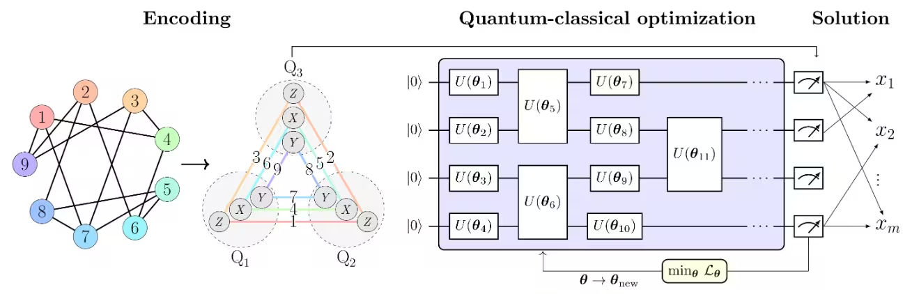In Abbildung 1 aus [1] wird das Max-Cut-Problem als Beispiel zur Illustration des PCE-Ansatzes verwendet. Das Max-Cut-Problem mit $m=9$ Knoten wird in einen Pauli-Korrelationsraum kodiert, was das Optimierungsproblem als Korrelationsmatrix darstellt — genauer gesagt als Zweikörper-Pauli-Matrix-Korrelationen über $n=3$ Qubits $(Q_1, Q_2, Q_3)$ . Die Farben der Knoten geben den Pauli-String an, der für jeden kodierten Knoten verwendet wird. Zum Beispiel wird Knoten 1, der der binären Variable $x_1$ entspricht, durch den Erwartungswert von $Z_1 \otimes Z_2 \otimes I_3$ kodiert, während $x_8$ durch $I_1 \otimes Y_2 \otimes Y_3$ kodiert wird. Dies entspricht einer Komprimierung der $m$ Variablen des Problems in $n = O(m^{1/2})$ Qubits. Allgemeiner ausgedrückt ermöglichen $k$ -Körper-Korrelationen polynomielle Komprimierungen der Ordnung $k$ mit $k>1$ . Die gewählte Pauli-Menge besteht aus drei Teilmengen gegenseitig kommutierender Pauli-Strings, sodass alle $m$ Korrelationen experimentell mit nur drei Messeinstellungen geschätzt werden können.

Eine Verlustfunktion $\mathcal{L}$ der Pauli-Erwartungswerte, die die ursprüngliche Max-Cut-Zielfunktion nachahmt, wird konstruiert. Die Verlustfunktion wird dann mithilfe eines quanten-klassischen Optimierungslösers optimiert, wie dem Variational Quantum Eigensolver (VQE).

Sobald die Optimierung abgeschlossen ist, wird die Lösung zurück in den ursprünglichen Optimierungsraum dekodiert und liefert die optimale Max-Cut-Lösung.

Anforderungen

Stelle vor Beginn dieses Tutorials sicher, dass du Folgendes installiert hast:

Qiskit SDK v1.0 oder neuer, mit Unterstützung für Visualisierung
Qiskit Runtime v0.22 oder neuer (pip install qiskit-ibm-runtime)

Setup

# Added by doQumentation — required packages for this notebook
!pip install -q networkx numpy qiskit qiskit-aer qiskit-ibm-runtime rustworkx scipy

from itertools import combinations

import numpy as np
import rustworkx as rx
import networkx as nx

from scipy.optimize import minimize, OptimizeResult

from qiskit.circuit.library import efficient_su2
from qiskit.transpiler.preset_passmanagers import generate_preset_pass_manager
from qiskit.quantum_info import SparsePauliOp
from qiskit_ibm_runtime import EstimatorV2 as Estimator
from qiskit_ibm_runtime import QiskitRuntimeService
from qiskit_ibm_runtime import Session
from rustworkx.visualization import mpl_draw
from qiskit_aer import AerSimulator

def calc_cut_size(graph, partition0, partition1):
    """Calculate the cut size of the given partitions of the graph."""

    cut_size = 0
    for edge0, edge1 in graph.edge_list():
        if edge0 in partition0 and edge1 in partition1:
            cut_size += 1
        elif edge0 in partition1 and edge1 in partition0:
            cut_size += 1
    return cut_size

Kleinskaliges Simulatorbeispiel

service = QiskitRuntimeService()
real_backend = service.least_busy(
    operational=True, simulator=False, min_num_qubits=156
)
backend = AerSimulator.from_backend(real_backend)
print(f"We are using the {backend.name}")

We are using the aer_simulator_from(ibm_pittsburgh)

Schritt 1: Klassische Eingaben auf ein Quantenproblem abbilden

Das Max-Cut-Problem

Das Max-Cut-Problem ist ein kombinatorisches Optimierungsproblem, das auf einem Graphen $G = (V, E)$ definiert ist, wobei $V$ die Menge der Knoten und $E$ die Menge der Kanten ist. Das Ziel ist es, die Knoten in zwei Mengen $S$ und $V \setminus S$ aufzuteilen, sodass die Anzahl der Kanten zwischen den beiden Mengen maximiert wird. Eine ausführliche Beschreibung des Max-Cut-Problems findest du im Tutorial zum Quantum Approximate Optimization Algorithm. Das Max-Cut-Problem wird auch als Beispiel im Tutorial Fortgeschrittene Techniken für QAOA verwendet. In diesen Tutorials wird der QAOA-Algorithmus zur Lösung des Max-Cut-Problems verwendet.

Graph -> Hamiltonian

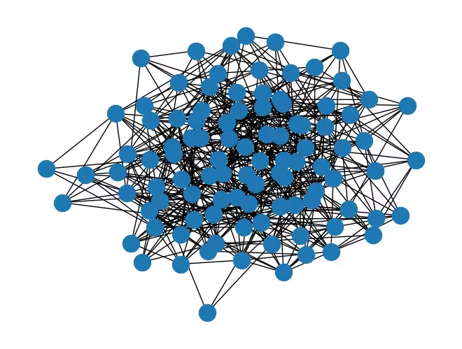
Betrachten wir zunächst einen zufälligen Graphen mit 100 Knoten.

num_nodes = 100  # Number of nodes in graph
seed = 42
graph = rx.undirected_gnp_random_graph(num_nodes, 0.1, seed=seed)
mpl_draw(graph)

Ausgabe der vorherigen Code-Zelle

nx_graph = nx.Graph()
nx_graph.add_nodes_from(range(num_nodes))

for edge in graph.edge_list():
    nx_graph.add_edge(edge[0], edge[1])

curr_cut_size, partition = nx.approximation.one_exchange(nx_graph, seed=1)
print(f"Initial cut size: {curr_cut_size}")

Initial cut size: 345

Wir kodieren den Graphen mit 100 Knoten in Zweikörper-Pauli-Matrix-Korrelationen über neun Qubits (siehe Erklärung unten). Der Graph wird als Korrelationsmatrix dargestellt, wobei jeder Knoten durch einen Pauli-String kodiert wird. Das Vorzeichen des Erwartungswerts des Pauli-Strings gibt die Partition des Knotens an. Zum Beispiel wird Knoten 0 durch einen Pauli-String $\prod_0 = I_{8} \otimes ... I_2 \otimes X_1 \otimes X_0$ kodiert. Das Vorzeichen des Erwartungswerts dieses Pauli-Strings gibt die Partition von Knoten 0 an. Wir definieren eine Pauli-Korrelationskodierung (PCE) relativ zu $\prod$ als

$x_i \coloneqq \textit{sgn}(\langle\prod_i \rangle),$

wobei $x_i$ die Partition von Knoten $i$ ist und $\langle \prod_i \rangle \coloneqq \langle \psi |\prod_i| \psi \rangle$ der Erwartungswert des den Knoten $i$ kodierenden Pauli-Strings über einen Quantenzustand $|\psi \rangle$ ist. Jetzt wollen wir den Graphen mithilfe von PCE in einen Hamiltonian kodieren. Wir unterteilen die Knoten in drei Mengen: $S_1$ , $S_2$ und $S_3$ . Dann kodieren wir die Knoten in jeder Menge mit den Pauli-Strings $X$ , $Y$ bzw. $Z$ . Wir müssen eine Beziehung zwischen der Anzahl der Knoten und der Anzahl der Qubits extrahieren, die wir benötigen, um alle Knoten zu kodieren. Die Verwendung aller möglichen Permutationen für die Kodierung ergibt:

m=3\binom{n}{k}.

In diesem Beispiel betrachten wir $k=2$ , daher gilt:

m = \frac{3}{2} n(n-1).

Die Anzahl der Qubits $n$ , die benötigt werden, um eine bestimmte Anzahl von Knoten $m$ auszudrücken, berechnet sich also zu:

n = \left\lceil \frac{1 + \sqrt{1 + \tfrac{8}{3}m}}{2} \right\rceil.

Das Symbol $\lceil \cdot \rceil$ steht für die Deckenfunktion (ceiling function), die jede reelle Zahl auf die nächste ganze Zahl aufrundet. Dadurch wird sichergestellt, dass die Anzahl der Qubits eine ganze Zahl ist.

num_qubits = int(np.ceil((1 + np.sqrt(1 + (8 / 3) * num_nodes)) / 2))

list_size = num_nodes // 3
node_x = [i for i in range(list_size)]
node_y = [i for i in range(list_size, 2 * list_size)]
node_z = [i for i in range(2 * list_size, num_nodes)]

print(f"Number of qubits: {num_qubits}")
print("List 1:", node_x)
print("List 2:", node_y)
print("List 3:", node_z)

Number of qubits: 9
List 1: [0, 1, 2, 3, 4, 5, 6, 7, 8, 9, 10, 11, 12, 13, 14, 15, 16, 17, 18, 19, 20, 21, 22, 23, 24, 25, 26, 27, 28, 29, 30, 31, 32]
List 2: [33, 34, 35, 36, 37, 38, 39, 40, 41, 42, 43, 44, 45, 46, 47, 48, 49, 50, 51, 52, 53, 54, 55, 56, 57, 58, 59, 60, 61, 62, 63, 64, 65]
List 3: [66, 67, 68, 69, 70, 71, 72, 73, 74, 75, 76, 77, 78, 79, 80, 81, 82, 83, 84, 85, 86, 87, 88, 89, 90, 91, 92, 93, 94, 95, 96, 97, 98, 99]

def build_pauli_correlation_encoding(pauli, node_list, n, k=2):
    pauli_correlation_encoding = []
    for idx, c in enumerate(combinations(range(n), k)):
        if idx >= len(node_list):
            break
        paulis = ["I"] * n
        paulis[c[0]], paulis[c[1]] = pauli, pauli
        pauli_correlation_encoding.append(("".join(paulis)[::-1], 1))

    hamiltonian = []
    for pauli, weight in pauli_correlation_encoding:
        hamiltonian.append(SparsePauliOp.from_list([(pauli, weight)]))

    return hamiltonian

pauli_correlation_encoding_x = build_pauli_correlation_encoding(
    "X", node_x, num_qubits
)
pauli_correlation_encoding_y = build_pauli_correlation_encoding(
    "Y", node_y, num_qubits
)
pauli_correlation_encoding_z = build_pauli_correlation_encoding(
    "Z", node_z, num_qubits
)

Schritt 2: Problem für die Ausführung auf Quantenhardware optimieren

Quantenschaltkreis

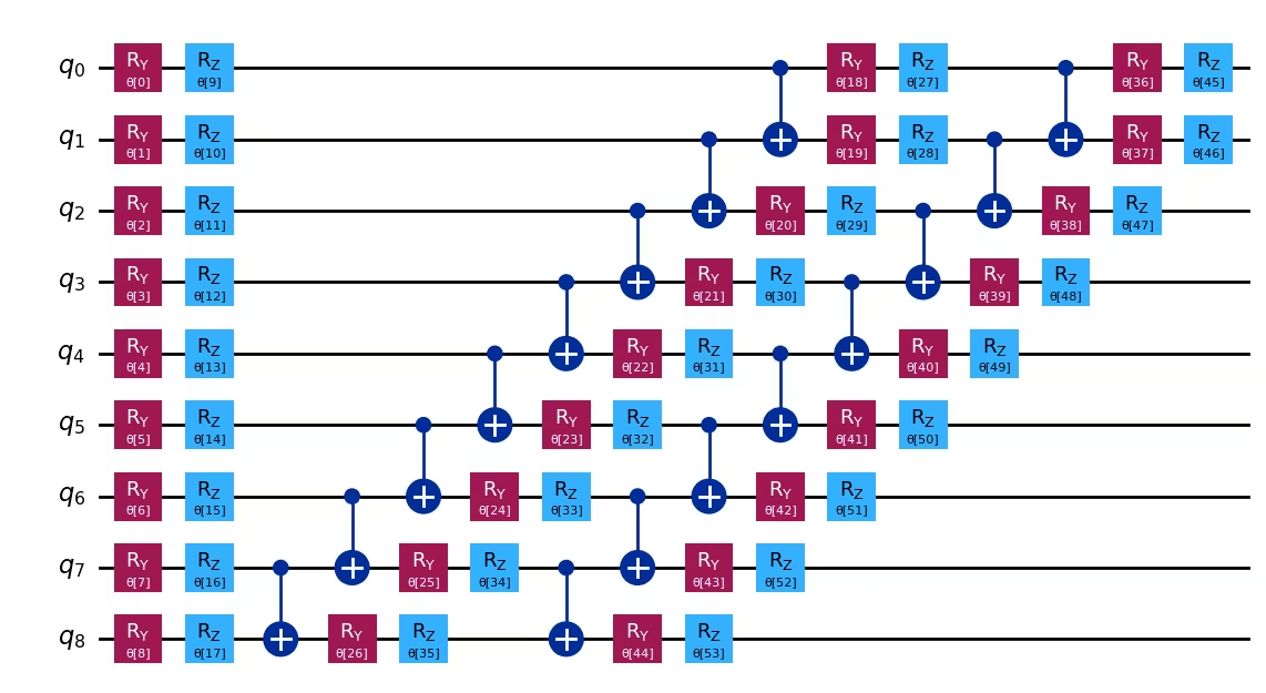
Hier wird der Zustand $|\psi \rangle$ mit $\mathbf{\theta}$ parametrisiert, und wir optimieren diese Parameter $\mathbf{\theta}$ mithilfe eines Variationsansatzes. Dieses Tutorial verwendet den efficient_su2-Ansatz für unseren Variationsalgorithmus aufgrund seiner Ausdrucksstärke und Einfachheit der Implementierung. Wir verwenden außerdem die relaxierte Verlustfunktion, die später in diesem Tutorial vorgestellt wird. Dadurch können wir groß angelegte Probleme mit weniger Qubits und flacheren Schaltkreistiefen angehen.

# Build the quantum circuit
qc = efficient_su2(num_qubits, su2_gates=["ry", "rz"], reps=2)
qc.draw("mpl")

Ausgabe der vorherigen Code-Zelle

# Optimize the circuit

pm = generate_preset_pass_manager(optimization_level=3, backend=backend)
qc = pm.run(qc)

Verlustfunktion

Für die Verlustfunktion $\mathcal{L}$ verwenden wir eine Relaxierung der Max-Cut-Zielfunktion, wie in [1] beschrieben, die als $\mathcal{V}(\mathbf{x}) \coloneqq \sum_{(i, j) \in E} W_{i, j}(1-x_i x_j)$ definiert ist. Hierbei bezeichnet $W_{i, j}$ das Gewicht der Kante $(i, j)$ und $x_i$ die Partition von Knoten $i$ . Die Verlustfunktion $\mathcal{L}$ ist gegeben durch:

$\mathcal{L}\coloneqq \sum_{(i, j) \in E} W_{i, j} \text{tanh} (\alpha \langle\prod_i \rangle) \text{tanh} (\alpha \langle\prod_j \rangle) + \mathcal{L}^{(\text{reg})},$

wobei die Max-Cut-Zielfunktion durch die glatten hyperbolischen Tangens der Erwartungswerte der die Knoten kodierenden Pauli-Strings ersetzt wird. Der Regularisierungsterm $\mathcal{L}^{(\text{reg})}$ und der Reskalierungsfaktor $\alpha$ , proportional zur Anzahl der Qubits, werden eingeführt, um die Leistung des Lösers zu verbessern.

Der Regularisierungsterm ist definiert als:

$\mathcal{L}^{(\text{reg})}$ ist definiert als $\mathcal{L}^{(\text{reg})} \coloneqq \beta \nu \lbrack \frac{1}{m} \sum_{i \in V} \text{tanh} (\alpha \langle\prod_i \rangle)^2 \rbrack ^2$

wobei $\beta=1/2$ , $\nu = |E|/2 + (m -1) /4$ , $|E|$ die Anzahl der Kanten und $m$ die Anzahl der Knoten im Graphen ist.

def loss_func_estimator(x, ansatz, hamiltonian, estimator, graph):
    """
    Calculates the specified loss function for the given ansatz, Hamiltonian, and graph.

    The expectation values of each Pauli string in the Hamiltonian are first obtained
    by running the ansatz on the quantum backend. These expectation values are then
    passed through the nonlinear function tanh(alpha * prod_i). The loss function is
    subsequently computed from these transformed values.
    """
    job = estimator.run(
        [
            (ansatz, hamiltonian[0], x),
            (ansatz, hamiltonian[1], x),
            (ansatz, hamiltonian[2], x),
        ]
    )
    result = job.result()

    # calculate the loss function
    node_exp_map = {}
    idx = 0
    for r in result:
        for ev in r.data.evs:
            node_exp_map[idx] = ev
            idx += 1

    loss = 0
    alpha = num_qubits
    for edge0, edge1 in graph.edge_list():
        loss += np.tanh(alpha * node_exp_map[edge0]) * np.tanh(
            alpha * node_exp_map[edge1]
        )

    regulation_term = 0
    for i in range(len(graph.nodes())):
        regulation_term += np.tanh(alpha * node_exp_map[i]) ** 2
    regulation_term = regulation_term / len(graph.nodes())
    regulation_term = regulation_term**2
    beta = 1 / 2
    v = len(graph.edges()) / 2 + (len(graph.nodes()) - 1) / 4
    regulation_term = beta * v * regulation_term

    loss = loss + regulation_term

    global experiment_result
    print(f"Iter {len(experiment_result)}: {loss}")
    experiment_result.append({"loss": loss, "exp_map": node_exp_map})
    return loss

Schritt 3: Ausführung mit Qiskit-Primitiven

In diesem Tutorial setzen wir max_iter=50 in der Optimierungsschleife zu Demonstrationszwecken. Wenn wir die Anzahl der Iterationen erhöhen, können wir bessere Ergebnisse erwarten.

pce = []
pce.append(
    [op.apply_layout(qc.layout) for op in pauli_correlation_encoding_x]
)
pce.append(
    [op.apply_layout(qc.layout) for op in pauli_correlation_encoding_y]
)
pce.append(
    [op.apply_layout(qc.layout) for op in pauli_correlation_encoding_z]
)

max_iter = 50
counter = {"i": 0}
last_x = {"value": None}
last_fun = {"value": None}

with Session(backend=backend) as session:
    estimator = Estimator(mode=session)

    experiment_result = []

    def loss_func(x):
        last_x["value"] = x.copy()
        if counter["i"] + 1 > max_iter:
            return last_fun["value"]
        counter["i"] += 1
        val = loss_func_estimator(
            x, qc, [pce[0], pce[1], pce[2]], estimator, graph
        )
        last_fun["value"] = val
        return val

    np.random.seed(seed)
    initial_params = np.random.rand(qc.num_parameters)

    result = minimize(
        loss_func, initial_params, method="COBYLA", options={"rhobeg": 1.0}
    )

    if counter["i"] >= max_iter:
        result = OptimizeResult(
            message=f"Return from COBYLA because the objective function has been evaluated {max_iter} times.",
            success=False,
            status=3,
            fun=last_fun["value"],
            x=last_x["value"],
            nfev=counter["i"],
        )

print(result)

Iter 0: 159.88755362682548
Iter 1: 113.46202580636677
Iter 2: 56.76494226400048
Iter 3: 32.63357946896002
Iter 4: 21.517837239610117
Iter 5: 30.96034960483569
Iter 6: 20.780475923938027
Iter 7: 24.54251816279811
Iter 8: 27.834486461763042
Iter 9: 16.705460776812693
Iter 10: 18.020587887236864
Iter 11: 12.252379762741352
Iter 12: 5.253885750886939
Iter 13: 6.985984759592262
Iter 14: 6.908717244584757
Iter 15: 12.915466016863858
Iter 16: 4.105776920457279
Iter 17: 11.707504530740305
Iter 18: 7.154360511076546
Iter 19: 10.3890865704735
Iter 20: 10.376147647857252
Iter 21: 2.533430195296697
Iter 22: 3.8612421907795462
Iter 23: 6.103735057461906
Iter 24: -1.1190368234312347
Iter 25: 6.125915279494738
Iter 26: 11.086280445482455
Iter 27: 10.102569882302827
Iter 28: -0.02664415648133822
Iter 29: 7.621887727398785
Iter 30: 5.967346615554497
Iter 31: 3.85345716014828
Iter 32: 4.5494846149011
Iter 33: 10.006668112637232
Iter 34: -3.1927138938527877
Iter 35: 2.8829882366285116
Iter 36: 3.3130087521654144
Iter 37: -4.907566569808272
Iter 38: -4.980134722109894
Iter 39: -2.990457463896541
Iter 40: -5.938401817344579
Iter 41: -2.1807712386469724
Iter 42: -1.0945774380342126
Iter 43: -4.7548102593556685
Iter 44: -3.8762362299208144
Iter 45: -4.9348321021624
Iter 46: -6.487722842864011
Iter 47: 0.7064210113389331
Iter 48: -2.3428323031772216
Iter 49: -2.626032270380895
 message: Return from COBYLA because the objective function has been evaluated 50 times.
 success: False
  status: 3
     fun: -2.626032270380895
       x: [ 1.375e+00  1.951e+00 ...  9.395e-01  8.948e-01]
    nfev: 50

Schritt 4: Nachbearbeitung und Rückgabe des Ergebnisses im gewünschten klassischen Format

Die Partitionen der Knoten werden durch Auswertung des Vorzeichens der Erwartungswerte der Pauli-Strings bestimmt, die die Knoten kodieren.

# Calculate the partitions based on the final expectation values
# If the expectation value is positive, the node belongs to partition 0 (par0)
# Otherwise, the node belongs to partition 1 (par1)
def get_partitions(experiment_result):
    par0, par1 = set(), set()
    best_index = min(
        range(len(experiment_result)),
        key=lambda i: experiment_result[i]["loss"],
    )
    for i in experiment_result[best_index]["exp_map"]:
        if experiment_result[best_index]["exp_map"][i] >= 0:
            par0.add(i)
        else:
            par1.add(i)
    return par0, par1, best_index

par0, par1, best_index = get_partitions(experiment_result)
print(par0, par1)

{0, 2, 3, 8, 9, 11, 12, 13, 17, 18, 20, 22, 23, 24, 25, 26, 27, 30, 35, 37, 38, 40, 43, 46, 48, 49, 50, 51, 53, 57, 61, 62, 63, 66, 67, 68, 70, 71, 74, 77, 81, 82, 83, 84, 87, 88, 94, 96, 99} {1, 4, 5, 6, 7, 10, 14, 15, 16, 19, 21, 28, 29, 31, 32, 33, 34, 36, 39, 41, 42, 44, 45, 47, 52, 54, 55, 56, 58, 59, 60, 64, 65, 69, 72, 73, 75, 76, 78, 79, 80, 85, 86, 89, 90, 91, 92, 93, 95, 97, 98}

Wir können die Schnittgröße des Max-Cut-Problems mithilfe der Partitionen der Knoten berechnen.

cut_size = calc_cut_size(graph, par0, par1)
print(f"Cut size: {cut_size}")

Cut size: 268

Sobald das Training abgeschlossen ist, führen wir eine Runde der Einzelbit-Austauschsuche durch, um die Lösung als klassischen Nachbearbeitungsschritt zu verbessern. Bei diesem Prozess tauschen wir die Partitionen zweier Knoten aus und bewerten die Schnittgröße. Wenn die Schnittgröße verbessert wird, behalten wir den Austausch. Wir wiederholen diesen Prozess für alle möglichen Knotenpaare, die durch eine Kante verbunden sind.

cur_bits = []

for i in experiment_result[best_index]["exp_map"]:
    if experiment_result[best_index]["exp_map"][i] >= 0:
        cur_bits.append(1)
    else:
        cur_bits.append(0)
print(cur_bits)

[1, 0, 1, 1, 0, 0, 0, 0, 1, 1, 0, 1, 1, 1, 0, 0, 0, 1, 1, 0, 1, 0, 1, 1, 1, 1, 1, 1, 0, 0, 1, 0, 0, 0, 0, 1, 0, 1, 1, 0, 1, 0, 0, 1, 0, 0, 1, 0, 1, 1, 1, 1, 0, 1, 0, 0, 0, 1, 0, 0, 0, 1, 1, 1, 0, 0, 1, 1, 1, 0, 1, 1, 0, 0, 1, 0, 0, 1, 0, 0, 0, 1, 1, 1, 1, 0, 0, 1, 1, 0, 0, 0, 0, 0, 1, 0, 1, 0, 0, 1]

# Swap the partitions and calculate the cut size

def swap_partitions(graph, cur_bits):
    best_cut = 0
    best_bits = []
    for edge0, edge1 in graph.edge_list():
        swapped_bits = cur_bits.copy()
        swapped_bits[edge0], swapped_bits[edge1] = (
            swapped_bits[edge1],
            swapped_bits[edge0],
        )

        cur_partition = [set(), set()]
        for i, bit in enumerate(swapped_bits):
            if bit > 0:
                cur_partition[0].add(i)
            else:
                cur_partition[1].add(i)
        cut_size = calc_cut_size(graph, cur_partition[0], cur_partition[1])
        if best_cut < cut_size:
            best_cut = cut_size
            best_bits = swapped_bits
    return best_cut, best_bits

best_cut, best_bits = swap_partitions(graph, cur_bits)
print(best_cut, best_bits)

279 [1, 0, 1, 1, 0, 0, 0, 0, 1, 0, 0, 1, 1, 1, 0, 0, 0, 1, 1, 0, 1, 0, 1, 1, 1, 1, 1, 1, 0, 0, 1, 0, 0, 0, 0, 1, 0, 1, 1, 0, 1, 0, 0, 1, 0, 0, 1, 0, 1, 1, 1, 1, 1, 1, 0, 0, 0, 1, 0, 0, 0, 1, 1, 1, 0, 0, 1, 1, 1, 0, 1, 1, 0, 0, 1, 0, 0, 1, 0, 0, 0, 1, 1, 1, 1, 0, 0, 1, 1, 0, 0, 0, 0, 0, 1, 0, 1, 0, 0, 1]

Großskaliges Hardware-Beispiel

# -------------------------Step 1-------------------------

num_nodes = 1500  # Number of nodes in graph
graph = rx.undirected_gnp_random_graph(num_nodes, 0.1, seed=seed)
nx_graph = nx.Graph()
nx_graph.add_nodes_from(range(num_nodes))
for edge in graph.edge_list():
    nx_graph.add_edge(edge[0], edge[1])

num_qubits = int(np.ceil((1 + np.sqrt(1 + (8 / 3) * num_nodes)) / 2))

list_size = num_nodes // 3
node_x = [i for i in range(list_size)]
node_y = [i for i in range(list_size, 2 * list_size)]
node_z = [i for i in range(2 * list_size, num_nodes)]

pauli_correlation_encoding_x = build_pauli_correlation_encoding(
    "X", node_x, num_qubits
)
pauli_correlation_encoding_y = build_pauli_correlation_encoding(
    "Y", node_y, num_qubits
)
pauli_correlation_encoding_z = build_pauli_correlation_encoding(
    "Z", node_z, num_qubits
)
print(f"We are using {num_qubits} qubits")

# -------------------------Step 2-------------------------
backend = real_backend
print(f"We are using the {backend.name}")
qc = efficient_su2(num_qubits, ["ry", "rz"], reps=2)
pm = generate_preset_pass_manager(optimization_level=3, backend=backend)
qc = pm.run(qc)
# -------------------------Step 3-------------------------
pce = []
pce.append(
    [op.apply_layout(qc.layout) for op in pauli_correlation_encoding_x]
)
pce.append(
    [op.apply_layout(qc.layout) for op in pauli_correlation_encoding_y]
)
pce.append(
    [op.apply_layout(qc.layout) for op in pauli_correlation_encoding_z]
)

# Run the optimization using a session.
max_iter = 50
counter = {"i": 0}
with Session(backend=backend) as session:
    estimator = Estimator(mode=session)
    estimator.options.environment.job_tags = ["TUT_PCEFQ"]
    experiment_result = []

    def loss_func(x):
        last_x["value"] = x.copy()
        if counter["i"] + 1 > max_iter:
            return last_fun["value"]
        counter["i"] += 1
        val = loss_func_estimator(
            x, qc, [pce[0], pce[1], pce[2]], estimator, graph
        )
        last_fun["value"] = val
        return val

    np.random.seed(seed)
    initial_params = np.random.rand(qc.num_parameters)
    result = minimize(
        loss_func, initial_params, method="COBYLA", options={"rhobeg": 1.0}
    )
    if counter["i"] >= max_iter:
        result = OptimizeResult(
            message=f"Return from COBYLA because the objective function has been evaluated {max_iter} times.",
            success=False,
            status=3,
            fun=last_fun["value"],
            x=last_x["value"],
            nfev=counter["i"],
        )
print(result)

# -------------------------Step 4-------------------------

par0, par1, best_index = get_partitions(experiment_result)
cut_size = calc_cut_size(graph, par0, par1)
print(f"Cut size: {cut_size}")

best_bits = []
cur_bits = []
for i in experiment_result[best_index]["exp_map"]:
    if experiment_result[best_index]["exp_map"][i] >= 0:
        cur_bits.append(1)
    else:
        cur_bits.append(0)
best_cut, best_bits = swap_partitions(graph, cur_bits)
# Print final solution

print(
    f"The best max-cut value achieved for a graph with {num_nodes} nodes on {num_qubits} qubits is {best_cut}"
)
print(f"and the specific partition we obtained is {best_bits}")

We are using 33 qubits
We are using the ibm_pittsburgh
Iter 0: 57399.57543902076
Iter 1: 56458.787143794
Iter 2: 40778.45608998947
Iter 3: 35571.58511146131
Iter 4: 33861.6835761173
Iter 5: 39697.22637736274
Iter 6: 34984.77893767163
Iter 7: 32051.882157096858
Iter 8: 26134.153216063707
Iter 9: 24914.322627065787
Iter 10: 24030.21227315425
Iter 11: 23047.463945514
Iter 12: 22629.42866110748
Iter 13: 17374.859132614685
Iter 14: 18020.11637762458
Iter 15: 17924.7066364044
Iter 16: 15825.1992250984
Iter 17: 16553.346711978447
Iter 18: 12393.565736512377
Iter 19: 11994.021456089155
Iter 20: 11199.994322735669
Iter 21: 9624.895532927634
Iter 22: 9073.811130188606
Iter 23: 9836.721241931278
Iter 24: 10555.925186133794
Iter 25: 9179.1179493286
Iter 26: 8495.394826965305
Iter 27: 8913.688189840399
Iter 28: 7830.448471810181
Iter 29: 7757.430542422075
Iter 30: 6796.187594518731
Iter 31: 7307.985913766867
Iter 32: 7340.225833330675
Iter 33: 7064.731899380469
Iter 34: 7632.270657372515
Iter 35: 7049.154710767935
Iter 36: 7486.118442084411
Iter 37: 6302.12602219333
Iter 38: 6244.934230209166
Iter 39: 7154.9748739261395
Iter 40: 6482.109600054041
Iter 41: 5718.475169152395
Iter 42: 5693.008457857462
Iter 43: 4869.782667921923
Iter 44: 4957.625304450959
Iter 45: 5582.240637063214
Iter 46: 4983.90082772116
Iter 47: 5416.268575648202
Iter 48: 4809.98398457807
Iter 49: 5092.527306646118
 message: Return from COBYLA because the objective function has been evaluated 50 times.
 success: False
  status: 3
     fun: 5092.527306646118
       x: [ 1.375e+00  1.951e+00 ...  7.259e-01  8.971e-01]
    nfev: 50
Cut size: 56152
The best max-cut value achieved for a graph with 1500 nodes on 33 qubits is 56219
and the specific partition we obtained is [1, 0, 0, 0, 1, 1, 0, 1, 1, 0, 0, 0, 0, 0, 1, 1, 0, 1, 0, 0, 1, 0, 0, 1, 1, 1, 0, 1, 1, 0, 1, 0, 1, 1, 0, 0, 0, 0, 0, 1, 0, 1, 0, 0, 1, 0, 0, 0, 1, 0, 1, 1, 1, 1, 0, 1, 0, 0, 1, 0, 0, 0, 0, 1, 1, 0, 0, 0, 0, 1, 1, 1, 1, 1, 0, 0, 0, 1, 0, 0, 1, 1, 0, 0, 1, 1, 1, 1, 1, 1, 0, 0, 0, 1, 0, 0, 0, 0, 1, 0, 1, 1, 1, 1, 1, 0, 1, 0, 0, 1, 0, 0, 0, 0, 0, 0, 1, 0, 0, 0, 1, 0, 1, 1, 1, 1, 0, 1, 1, 1, 1, 0, 0, 0, 1, 0, 0, 0, 1, 1, 0, 1, 1, 0, 1, 0, 0, 1, 1, 1, 1, 1, 1, 0, 1, 0, 1, 0, 0, 0, 0, 0, 0, 1, 0, 1, 0, 0, 1, 1, 1, 0, 1, 0, 1, 0, 0, 1, 1, 0, 1, 0, 1, 0, 0, 0, 1, 0, 1, 0, 1, 1, 1, 1, 1, 0, 1, 0, 1, 1, 1, 1, 1, 1, 0, 0, 0, 0, 0, 1, 0, 1, 0, 0, 1, 1, 0, 0, 1, 0, 1, 0, 1, 0, 0, 0, 0, 0, 1, 1, 0, 0, 0, 0, 0, 1, 1, 0, 0, 1, 1, 1, 1, 1, 1, 1, 0, 1, 1, 1, 1, 0, 1, 1, 0, 1, 0, 0, 1, 1, 1, 0, 1, 0, 1, 1, 1, 0, 1, 0, 0, 0, 1, 1, 1, 1, 1, 1, 0, 1, 0, 0, 0, 0, 1, 1, 1, 1, 1, 1, 1, 0, 0, 1, 1, 1, 1, 0, 1, 0, 0, 1, 1, 1, 0, 1, 0, 1, 1, 1, 1, 0, 1, 1, 0, 1, 0, 0, 0, 0, 0, 0, 0, 0, 0, 0, 1, 0, 0, 0, 0, 0, 0, 1, 1, 1, 0, 0, 1, 1, 1, 0, 1, 0, 1, 0, 1, 0, 1, 1, 1, 0, 0, 1, 1, 1, 0, 1, 0, 0, 0, 1, 1, 1, 0, 0, 0, 1, 0, 1, 0, 0, 0, 0, 1, 1, 0, 0, 1, 1, 1, 1, 0, 1, 0, 1, 0, 0, 1, 1, 0, 0, 1, 1, 0, 0, 0, 1, 1, 1, 0, 1, 1, 0, 0, 0, 1, 1, 1, 0, 0, 1, 1, 1, 1, 1, 0, 0, 1, 1, 0, 0, 0, 0, 0, 0, 1, 1, 1, 1, 1, 1, 1, 0, 0, 0, 1, 1, 0, 0, 0, 1, 0, 0, 1, 0, 0, 1, 0, 1, 1, 0, 0, 0, 0, 0, 0, 0, 1, 1, 1, 1, 1, 0, 0, 0, 1, 0, 0, 1, 1, 1, 1, 1, 1, 1, 1, 1, 1, 1, 0, 1, 0, 1, 1, 1, 1, 1, 0, 0, 0, 1, 1, 1, 0, 1, 1, 1, 1, 0, 0, 1, 0, 1, 0, 1, 1, 0, 0, 0, 1, 0, 1, 0, 1, 1, 1, 0, 1, 0, 1, 1, 0, 1, 1, 0, 1, 1, 1, 0, 0, 1, 1, 1, 0, 1, 0, 1, 0, 1, 0, 0, 0, 1, 1, 0, 1, 0, 0, 1, 0, 0, 1, 0, 0, 0, 0, 0, 1, 0, 0, 0, 0, 0, 1, 0, 0, 0, 0, 0, 0, 0, 0, 1, 0, 1, 0, 0, 1, 0, 1, 0, 0, 0, 0, 1, 0, 0, 0, 1, 1, 1, 1, 1, 0, 0, 1, 0, 1, 1, 1, 1, 0, 1, 1, 0, 1, 0, 0, 0, 0, 1, 0, 0, 1, 1, 0, 1, 0, 1, 0, 1, 0, 0, 1, 0, 0, 0, 1, 1, 1, 0, 0, 1, 0, 0, 1, 0, 1, 0, 1, 1, 1, 1, 0, 1, 1, 1, 0, 1, 1, 1, 1, 1, 1, 1, 1, 0, 1, 0, 1, 1, 1, 0, 0, 0, 1, 0, 0, 0, 0, 0, 1, 0, 0, 1, 0, 1, 1, 1, 0, 0, 0, 0, 0, 0, 1, 0, 1, 1, 0, 1, 1, 1, 1, 0, 0, 1, 1, 0, 1, 1, 1, 0, 1, 0, 1, 0, 1, 0, 0, 0, 0, 0, 0, 0, 0, 1, 0, 0, 1, 1, 1, 0, 1, 1, 0, 0, 0, 1, 0, 1, 0, 1, 1, 1, 0, 1, 1, 1, 0, 1, 1, 1, 1, 0, 0, 1, 1, 0, 1, 1, 1, 0, 0, 0, 0, 0, 0, 0, 1, 1, 1, 1, 1, 0, 1, 0, 1, 0, 1, 0, 0, 0, 1, 0, 1, 0, 1, 0, 1, 0, 1, 0, 1, 1, 1, 1, 1, 0, 0, 1, 0, 1, 0, 1, 0, 1, 1, 0, 1, 0, 1, 0, 0, 0, 1, 0, 0, 0, 1, 1, 1, 0, 1, 0, 0, 1, 0, 1, 0, 1, 0, 1, 0, 0, 1, 0, 1, 0, 0, 0, 1, 1, 1, 0, 1, 0, 0, 0, 0, 1, 0, 0, 0, 0, 1, 0, 0, 1, 1, 1, 0, 1, 1, 0, 1, 1, 1, 0, 0, 0, 0, 1, 0, 1, 0, 0, 0, 1, 0, 1, 0, 1, 0, 0, 1, 0, 1, 0, 1, 0, 1, 1, 0, 0, 1, 1, 0, 1, 1, 0, 0, 1, 0, 1, 1, 1, 0, 1, 1, 0, 1, 1, 1, 0, 1, 1, 0, 1, 0, 1, 0, 1, 1, 0, 1, 1, 0, 1, 1, 0, 0, 0, 1, 0, 1, 0, 0, 0, 0, 0, 1, 0, 0, 1, 1, 0, 1, 0, 1, 1, 0, 1, 1, 0, 1, 1, 1, 1, 0, 1, 0, 1, 1, 0, 0, 1, 0, 0, 1, 1, 0, 1, 1, 1, 0, 1, 1, 0, 1, 1, 1, 0, 1, 0, 0, 0, 1, 0, 0, 1, 1, 1, 0, 0, 1, 0, 1, 1, 1, 0, 1, 0, 1, 1, 1, 1, 1, 1, 0, 1, 0, 0, 0, 1, 0, 1, 0, 1, 1, 0, 0, 0, 1, 1, 0, 1, 1, 1, 1, 1, 1, 1, 1, 1, 1, 1, 1, 0, 1, 1, 1, 0, 0, 0, 0, 1, 0, 0, 0, 0, 1, 1, 1, 0, 0, 1, 0, 0, 0, 0, 0, 0, 0, 1, 0, 0, 0, 0, 0, 0, 0, 1, 1, 0, 0, 1, 0, 0, 1, 1, 0, 1, 0, 1, 0, 1, 0, 0, 1, 1, 0, 1, 1, 1, 0, 0, 1, 1, 1, 1, 1, 0, 0, 1, 0, 1, 1, 1, 1, 0, 1, 0, 1, 1, 0, 0, 1, 0, 1, 0, 0, 1, 0, 1, 1, 1, 1, 1, 1, 1, 0, 1, 0, 1, 1, 0, 0, 0, 0, 0, 1, 1, 0, 0, 1, 1, 1, 1, 1, 1, 1, 1, 1, 1, 0, 1, 1, 1, 1, 0, 1, 0, 0, 0, 1, 1, 1, 1, 0, 0, 0, 1, 1, 0, 0, 0, 0, 0, 1, 0, 0, 0, 1, 0, 0, 0, 1, 1, 1, 1, 0, 0, 0, 1, 1, 1, 1, 1, 1, 1, 1, 1, 1, 0, 1, 1, 1, 1, 1, 1, 1, 0, 0, 0, 0, 0, 1, 1, 0, 0, 0, 1, 1, 0, 0, 0, 0, 0, 1, 0, 0, 0, 0, 0, 0, 0, 0, 1, 0, 1, 0, 1, 1, 1, 0, 1, 0, 1, 1, 1, 1, 1, 0, 1, 1, 1, 1, 0, 1, 1, 1, 1, 1, 1, 0, 0, 1, 1, 0, 0, 1, 1, 1, 1, 1, 0, 1, 0, 1, 1, 1, 1, 1, 0, 1, 0, 0, 1, 1, 0, 0, 0, 0, 1, 1, 1, 1, 0, 1, 1, 1, 1, 1, 1, 1, 1, 0, 0, 0, 1, 0, 1, 1, 0, 1, 0, 1, 1, 1, 1, 0, 1, 1, 1, 1, 1, 1, 1, 1, 0, 1, 1, 0, 0, 0, 0, 0, 0, 1, 1, 0, 0, 0, 0, 0, 0, 1, 0, 0, 0, 0, 0, 0, 0, 0, 0, 0, 1, 0, 0, 0, 0, 0, 0, 0, 1, 0, 0, 1, 0, 0, 0, 0, 0, 0, 0, 0, 0, 0, 0, 0, 0, 0, 1, 1, 1, 0, 1, 1, 1, 1, 1, 0, 1, 0, 1, 1, 0, 1, 1, 1, 1, 1, 1, 1, 1, 1, 1, 0, 1, 1, 1, 1, 1, 1, 1, 0, 1, 0, 1, 0, 1, 1, 1, 1, 1, 1, 1, 1, 1, 1, 0, 0, 1, 1, 1, 1, 0, 1, 0, 1, 1, 1, 1, 1, 1, 1, 0, 0, 1, 1, 1, 0, 0, 1, 0, 1, 1, 1, 1, 0, 1, 1, 1, 1, 1, 1, 0, 1, 1, 0, 1, 1, 0, 1, 1, 1, 1, 1, 1, 1, 1, 1, 0, 1, 1, 1, 1, 0, 1, 1, 1, 1, 1, 1, 1, 1, 1, 1, 1, 1, 1, 1, 1, 1, 1, 1, 1]

Nächste Schritte

Empfehlungen

Wenn du diese Arbeit interessant findest, könnte dich folgendes Material interessieren:

Referenzen

[1] Sciorilli, M., Borges, L., Patti, T. L., García-Martín, D., Camilo, G., Anandkumar, A., & Aolita, L. (2024). Towards large-scale quantum optimization solvers with few qubits. arXiv preprint arXiv:2401.09421.

Tutorial-Umfrage

Bitte nimm an dieser kurzen Umfrage teil, um Feedback zu diesem Tutorial zu geben. Deine Einblicke helfen uns, unsere Inhalte und die Benutzererfahrung zu verbessern.

Hinweis: Diese Umfrage stammt von IBM Quantum und bezieht sich auf den Tutorial-Inhalt (geschrieben von IBM). doQumentation stellt die Website, Übersetzungen und Code-Ausführung bereit — für Feedback dazu bitte ein GitHub-Issue öffnen.

Lernziele​

Voraussetzungen​

Hintergrund​

Überblick​

Anforderungen​

Setup​

Kleinskaliges Simulatorbeispiel​

Schritt 1: Klassische Eingaben auf ein Quantenproblem abbilden​

Das Max-Cut-Problem​

Graph -> Hamiltonian​

Schritt 2: Problem für die Ausführung auf Quantenhardware optimieren​

Quantenschaltkreis​

Verlustfunktion​

Schritt 3: Ausführung mit Qiskit-Primitiven​

Schritt 4: Nachbearbeitung und Rückgabe des Ergebnisses im gewünschten klassischen Format​