Warm-Start-QAOA mit dem Optimization Mapper Qiskit-Addon

Geschätzte Nutzungsdauer: 9 Minuten auf einem Heron r3 (HINWEIS: Dies ist nur eine Schätzung. Deine tatsächliche Laufzeit kann abweichen.)

Lernziele

• Wie du ein Max-Cut-Problem mithilfe von qiskit-addon-opt-mapper auf eine quantenbasierte Quadratic-Unconstrained-Binary-Optimization-Formulierung (QUBO) abbildest

• Wie du Standard-QAOA implementierst und auf einem Simulator ausführst

• Wie du WS-QAOA anwendest, indem du die Relaxation des quadratischen Programms (QP) berechnest und den Warmstart-Circuit erstellst

• Wie du die Energiekonvergenz und Lösungsqualität zwischen Standard QAOA und WS-QAOA vergleichst

Voraussetzungen

• QAOA-Tutorial

• Fortgeschrittenes QAOA-Tutorial

Hintergrund

Der Quantum Approximate Optimization Algorithm (QAOA) ist ein hybrider quanten-klassischer Algorithmus, der zur Lösung kombinatorischer Optimierungsprobleme wie Max-Cut und allgemeiner QUBO-Formulierungen entwickelt wurde. Eine grundlegende Einführung in QAOA mit Qiskit findest du im QAOA-Tutorial; fortgeschrittenere Techniken zum Circuit-Aufbau findest du im fortgeschrittenen QAOA-Tutorial.

Im Standard-QAOA gilt:

• Der Anfangszustand ist die gleichverteilte Überlagerung $|+\rangle^{\otimes n}$.
• Variationelle Parameter werden zufällig initialisiert.
• Ein klassischer Optimierer sucht nach Parametern, die die Kostenfunktion minimieren.

Bei praktischen Problemgrößen und verrauschter Quantenhardware kann eine zufällige Initialisierung jedoch zu langsamer Konvergenz, schlechten lokalen Minima und erhöhten Optimierungskosten führen.

Warm-Start-QAOA (WS-QAOA) verbessert dies, indem Erkenntnisse aus der klassischen Optimierung direkt in den Quanten-Circuit einfließen. Dieses Tutorial folgt den Methoden, die von Egger, Mareček und Woerner in Warm-starting quantum optimization vorgestellt wurden. Die zentrale Idee besteht darin:

1. Eine kontinuierliche Relaxierung lösen des ursprünglichen binären Problems (ein quadratisches Programm über $[0,1]^n$ statt $\{0,1\}^n$).

2. Die relaxierte Lösung $c^*_i \in [0,1]$ in einen benutzerdefinierten Anfangszustand codieren, indem $Y$-Rotationswinkel $\theta_i = 2\arcsin(\sqrt{c^*_i})$ verwendet werden, sodass Qubit $i$ in einem Zustand startet, dessen Wahrscheinlichkeit, $|1\rangle$ zu messen, $c^*_i$ ist.

3. Den standardmäßigen $X$-Mixer ersetzen durch einen benutzerdefinierten Mixer, dessen Grundzustand der Warm-Start-Anfangszustand ist, sodass der Algorithmus in der Nähe der klassischen Lösung startet und die Umgebung erkunden kann.

Ein Regularisierungsparameter $\varepsilon \in [0, 0.5]$ begrenzt $c^*_i$ auf einen Bereich fern von 0 und 1, um Erreichbarkeitsprobleme zu vermeiden; Qubits, die in $|0\rangle$ oder $|1\rangle$ initialisiert werden, können vom Kosten-Hamiltonian nicht bewegt werden. Bei $\varepsilon = 0.5$ reduziert sich WS-QAOA exakt auf Standard-QAOA.

Die Problemmodellierung verwendet das Paket qiskit-addon-opt-mapper, dessen Anwendungsklasse Maxcut die QUBO direkt aus einem Graphen erstellt, und dessen Konverter und Übersetzer das resultierende Problem auf Quanten-Hamiltonians abbilden.

Anforderungen

Bevor du mit diesem Tutorial beginnst, stelle sicher, dass Folgendes installiert ist:

• Qiskit SDK v2.0 oder höher, mit Unterstützung für Visualisierung

• Qiskit Runtime v0.43 oder höher (pip install qiskit-ibm-runtime)

• Optimization Mapper Qiskit-Addon (pip install qiskit-addon-opt-mapper)

• SciPy (pip install scipy)

• NetworkX (pip install networkx)

Setup

Importiere alle benötigten Bibliotheken und definiere Hilfsfunktionen, die im gesamten Tutorial verwendet werden.

# Added by doQumentation — required packages for this notebook
!pip install -q matplotlib networkx numpy qiskit qiskit-addon-opt-mapper qiskit-ibm-runtime scipy

import numpy as np
import matplotlib.pyplot as plt
import networkx as nx
from scipy.optimize import minimize

from qiskit.circuit import QuantumCircuit, ParameterVector
from qiskit.circuit.library import qaoa_ansatz
from qiskit.quantum_info import Statevector
from qiskit.primitives import StatevectorEstimator, StatevectorSampler
from qiskit.transpiler.preset_passmanagers import generate_preset_pass_manager
from qiskit_ibm_runtime import (
    QiskitRuntimeService,
    Session,
    EstimatorOptions,
    EstimatorV2 as Estimator,
    SamplerV2 as Sampler,
)

from qiskit_addon_opt_mapper.applications import Maxcut
from qiskit_addon_opt_mapper.converters import OptimizationProblemToQubo
from qiskit_addon_opt_mapper.translators import to_ising

Kleinskaliges Simulatorbeispiel

Wir verwenden als durchgängiges Beispiel ein kleines Max-Cut-Problem auf einem gewichteten Graphen. Max-Cut fragt: Finde für einen Graphen $G=(V,E)$ mit Kantengewichten $w_{ij}$ eine Partition der Knoten in zwei Mengen $S$ und $\bar{S}$, die das Gesamtgewicht der Kanten, die den Schnitt kreuzen, maximiert.

Als QUBO-Minimierungsproblem lässt sich Max-Cut wie folgt schreiben: $\min_{x \in \{0,1\}^n} -\sum_{(i,j) \in E} w_{ij}(x_i + x_j - 2x_i x_j)$

Wir arbeiten mit einem Graphen aus vier Knoten, um die Handhabbarkeit auf einem Simulator zu gewährleisten.

Schritt 1: Klassische Eingaben auf ein Quantenproblem abbilden

Wir definieren das Max-Cut-Problem mithilfe der Anwendungsklasse Maxcut aus qiskit-addon-opt-mapper, die die QUBO-Formulierung direkt aus einem Graphen erstellt. Anschließend wandeln wir es in eine QUBO um und übersetzen es in einen für QAOA geeigneten Ising-Hamiltonian (SparsePauliOp). Außerdem lösen wir die kontinuierliche Relaxierung der QUBO — indem wir die binäre Nebenbedingung $x_i \in \{0,1\}$ durch $x_i \in [0,1]$ ersetzen —, um den Warm-Start-Anfangspunkt $c^*$ zu erhalten.

# Define a 4-node weighted graph for the max-cut problem
n_nodes = 4
edges = [(0, 1, 1.0), (0, 2, 1.0), (1, 2, 1.0), (1, 3, 1.0), (2, 3, 1.0)]

G = nx.Graph()
G.add_nodes_from(range(n_nodes))
G.add_weighted_edges_from(edges)

pos = nx.spring_layout(G, seed=42)
edge_labels = {(u, v): d["weight"] for u, v, d in G.edges(data=True)}

fig, ax = plt.subplots(figsize=(4, 3))
nx.draw(G, pos, with_labels=True, node_color="lightblue", ax=ax)
nx.draw_networkx_edge_labels(G, pos, edge_labels=edge_labels, ax=ax)
ax.set_title("Max-Cut graph")
plt.tight_layout()
plt.show()

Der Graph hat fünf Kanten. Der optimale Max-Cut partitioniert die Knoten in $S = \{0, 3\}$ und $\bar{S} = \{1, 2\}$ (oder sein Komplement), wobei vier der fünf Kanten durchtrennt werden, was einem Cut-Wert von 4 entspricht.

# Build the max-cut problem directly from the NetworkX graph using the
# Maxcut application class. Internally it constructs the QUBO
#   minimize  -sum_{(i,j) in E} w_ij * (x_i + x_j - 2*x_i*x_j)
# (each edge contributes -w to the linear terms and +2w to the quadratic
# term), so we get the same OptimizationProblem without the boilerplate.
maxcut = Maxcut(G)
prob = maxcut.to_optimization_problem()
print(prob.prettyprint())

Problem name: Max-cut

Maximize
  -2*x_0*x_1 - 2*x_0*x_2 - 2*x_1*x_2 - 2*x_1*x_3 - 2*x_2*x_3 + 2*x_0 + 3*x_1
  + 3*x_2 + 2*x_3

Subject to
  No constraints

  Binary variables (4)
    x_0 x_1 x_2 x_3

Die Klasse Maxcut kapselt die QUBO-Konstruktion, sodass wir die Max-Cut-Zielfunktion nicht von Hand ausschreiben müssen. Die ausgegebene Zielfunktion zeigt den linearen Koeffizienten jeder Variable (wie viel sie einzeln zum Cut beiträgt) sowie den quadratischen Koeffizienten jedes Kreuzterms (die Strafe dafür, zwei benachbarte Knoten auf dieselbe Seite zu setzen). Das zugrunde liegende OptimizationProblem, das von to_optimization_problem() zurückgegeben wird, unterstützt binäre, ganzzahlige, kontinuierliche und Spin-Variablen und ist dasselbe Objekt, das von den im nächsten Schritt verwendeten Konvertern und Übersetzern erwartet wird.

# Convert the OptimizationProblem to a QUBO, then translate to an Ising Hamiltonian
#
# The substitution x_i = (1 - z_i)/2  maps binary variables to spin operators,
# yielding a Hamiltonian H_C = sum_i h_i Z_i + sum_{i<j} J_ij Z_i Z_j + constant.
# QAOA minimizes <H_C> to find the ground state, which encodes the optimal cut.
converter = OptimizationProblemToQubo()
qubo = converter.convert(prob)

cost_operator, offset = to_ising(qubo)
n_qubits = cost_operator.num_qubits

print(f"Cost Hamiltonian H_C ({n_qubits} qubits):")
print(cost_operator)
print(f"\nOffset (constant shift): {offset}")
print("  QUBO value = Ising energy + offset")

Cost Hamiltonian H_C (4 qubits):
SparsePauliOp(['IIZZ', 'IZIZ', 'IZZI', 'ZIZI', 'ZZII'],
              coeffs=[0.5+0.j, 0.5+0.j, 0.5+0.j, 0.5+0.j, 0.5+0.j])

Offset (constant shift): -2.5
  QUBO value = Ising energy + offset

Der Übersetzer to_ising gibt ein SparsePauliOp zurück, das $H_C$ darstellt, sowie einen skalaren offset, sodass $\text{QUBO value} = \langle H_C \rangle + \text{offset}$ gilt. Für dieses Max-Cut-Problem mit ausschließlich Einheitsgewichten gilt $h_i = 0$ für alle Qubits (der Graph ist nach der Substitution $x_i \to z_i$ in den linearen Termen symmetrisch), und jede Kante trägt eine $Z_i Z_j$-Kopplung der Stärke $+0.5$ bei. Der minimale Eigenwert von $H_C$ entspricht dem maximalen Cut.

# Solve the continuous (QP) relaxation to obtain the warm-start point c*
#
# The QP relaxation replaces the binary constraint x_i in {0,1} with x_i in [0,1]
# and minimizes the same quadratic objective. Its solution c*_i gives the
# probability that variable i should be 1 according to the classical relaxation.
#
# The max-cut QUBO has a non-convex quadratic matrix (negative eigenvalues),
# so the relaxed problem has multiple local minima. A naive single start from
# [0.5,...,0.5] converges to the symmetric saddle point c* = [0.5,...,0.5],
# which carries no useful structural information about the problem.
# Multi-start optimization is used to reliably find the global minimum.
Q = qubo.objective.quadratic.to_array(symmetric=True)
mu = qubo.objective.linear.to_array()

def qp_objective(x_cont):
    """Continuous relaxation of the QUBO objective."""
    return x_cont @ Q @ x_cont + mu @ x_cont + qubo.objective.constant

bounds = [(0.0, 1.0)] * n_qubits

rng = np.random.default_rng(42)
best_val = np.inf
c_star = None
for _ in range(200):
    x0 = rng.uniform(0.0, 1.0, n_qubits)
    result = minimize(qp_objective, x0, method="L-BFGS-B", bounds=bounds)
    if result.fun < best_val:
        best_val = result.fun
        c_star = result.x

print(f"QP relaxation solution c* = {np.round(c_star, 4)}")
print(f"QP objective value        = {best_val:.4f}")

QP relaxation solution c* = [1. 0. 0. 1.]
QP objective value        = -4.0000

Der Multi-Start-Solver findet $c^* = [1, 0, 0, 1]$ (oder sein Komplement $[0, 1, 1, 0]$), was die tatsächliche optimale binäre Lösung ist. Für dieses Problem ist die QP-Relaxierung eng (tight): Das kontinuierliche Minimum stimmt mit dem ganzzahligen Optimum überein, das heißt, die Relaxierung identifiziert sofort den besten Cut. Nach der Regularisierung mit $\varepsilon = 0.25$ in Schritt 2 wird diese Lösung in den Warm-Start-Anfangszustand codiert.

Schritt 2: Problem für die Ausführung auf Quantenhardware optimieren

Wir erstellen zwei QAOA-Circuits und bereiten die Warm-Start-Winkel aus der QP-Lösung vor.

Standard-QAOA verwendet die gleichverteilte Überlagerung $|+\rangle^{\otimes n}$ als Anfangszustand und den standardmäßigen $X$-Mixer $H_M = -\sum_i X_i$, implementiert als $\prod_i R_X(-2\beta)$ pro Schicht.

Warm-Start-QAOA (WS-QAOA) aus [1] nimmt zwei strukturelle Änderungen pro Qubit $i$ vor:

• Anfangszustand: $R_Y(\theta_i)|0\rangle$ mit $\theta_i = 2\arcsin(\sqrt{c^*_i})$, sodass die Wahrscheinlichkeit, $|1\rangle$ zu messen, $c^*_i$ entspricht.
• Benutzerdefinierter Mixer: $R_Y(\theta_i)\, R_Z(-2\beta)\, R_Y(-\theta_i)$, dessen Grundzustand $R_Y(\theta_i)|0\rangle$ ist. Das bedeutet, WS-QAOA startet im Grundzustand seines eigenen Mixers – dieselbe Eigenschaft, die Standard-QAOA mit $|+\rangle$ und dem $X$-Mixer erfüllt.

Hinweis zu Schichten: Bei p=1 (einer einzelnen QAOA-Schicht) ist Standard-QAOA auf Graphen mit Dreiecken (dieser Graph enthält das Dreieck 0-1-2) analytisch auf ~49 % der optimalen Energie beschränkt. Der Warm-Start umgeht diese Einschränkung, indem er Vorwissen über die Lösung direkt in den Anfangszustand codiert.

# Number of QAOA layers (each layer = one cost unitary + one mixer unitary)
p = 1

# Regularization: clip c* to [epsilon, 1-epsilon] so no qubit is initialized
# in |0> or |1>, which would freeze it under the cost Hamiltonian.
epsilon = 0.25

c_clipped = np.clip(c_star, epsilon, 1 - epsilon)
thetas = 2 * np.arcsin(np.sqrt(c_clipped))

print(f"Continuous relaxation c*  = {np.round(c_star, 4)}")
print(f"After regularization      = {np.round(c_clipped, 4)}")
print(f"Warm-start angles theta   = {np.round(thetas, 4)} radians")
print()
print("Angle interpretation:")
print("  theta = 0      <->  c* = 0   (qubit points toward |0>)")
print(
    "  theta = pi/2   <->  c* = 0.5 (qubit in equal superposition, like |+>)"
)
print("  theta = pi     <->  c* = 1   (qubit points toward |1>)")

Continuous relaxation c*  = [1. 0. 0. 1.]
After regularization      = [0.75 0.25 0.25 0.75]
Warm-start angles theta   = [2.0944 1.0472 1.0472 2.0944] radians

Angle interpretation:
  theta = 0      <->  c* = 0   (qubit points toward |0>)
  theta = pi/2   <->  c* = 0.5 (qubit in equal superposition, like |+>)
  theta = pi     <->  c* = 1   (qubit points toward |1>)

Nach dem Clipping wird $c^* = 1$ zu $1 - \varepsilon = 0.75$ und $c^* = 0$ zu $\varepsilon = 0.25$. Die resultierenden Winkel $\theta \approx [2.09, 1.05, 1.05, 2.09]$ Radiant rotieren die Qubits 0 und 3 stark in Richtung $|1\rangle$ und die Qubits 1 und 2 in Richtung $|0\rangle$, wodurch die Struktur des optimalen Cuts direkt in den anfänglichen Quantenzustand codiert wird.

def apply_cost_unitary(qc, cost_op, gamma):
    """Apply exp(-i * gamma * H_C) to the circuit.

    Each Pauli term in H_C contributes a rotation gate:
      - Single-Z term h_i * Z_i  ->  RZ(2 * gamma * h_i) on qubit i
      - Two-Z term J_ij * Z_i Z_j  ->  CNOT, RZ(2 * gamma * J_ij), CNOT
    """
    for pauli_term, coeff in zip(cost_op.paulis, cost_op.coeffs):
        indices = [
            j for j, q in enumerate(pauli_term.to_label()[::-1]) if q == "Z"
        ]
        if len(indices) == 1:
            qc.rz(2 * gamma * coeff.real, indices[0])
        elif len(indices) == 2:
            qc.cx(indices[0], indices[1])
            qc.rz(2 * gamma * coeff.real, indices[1])
            qc.cx(indices[0], indices[1])

def build_ws_qaoa(cost_op, n_layers, n_qubits, thetas):
    """WS-QAOA: warm-start initial state + custom per-qubit mixer.

    Per Egger et al. (2021) Eq. (1)-(2):
      Initial state per qubit i:  R_Y(theta_i) |0>
      Mixer gate per qubit i:     R_Y(theta_i) R_Z(-2*beta) R_Y(-theta_i)
    """
    gammas = ParameterVector("γ", n_layers)
    betas = ParameterVector("β", n_layers)
    qc = QuantumCircuit(n_qubits)
    for i, theta in enumerate(thetas):
        qc.ry(theta, i)  # warm-start initial state
    for k in range(n_layers):
        apply_cost_unitary(qc, cost_op, gammas[k])
        for i, theta in enumerate(thetas):
            qc.ry(theta, i)
            qc.rz(-2 * betas[k], i)
            qc.ry(-theta, i)
    return qc, gammas, betas

# Standard QAOA via the Qiskit built-in helper:
# qaoa_ansatz prepares |+>^n, then alternates exp(-i*gamma*H_C) with the
# default X-mixer for `reps` layers. The returned circuit exposes the
# variational parameters via std_qc.parameters.
std_qc = qaoa_ansatz(cost_operator, reps=p)

# WS-QAOA: keep the custom builder. The per-qubit mixer
# R_Y(theta_i) R_Z(-2*beta) R_Y(-theta_i) is implemented as an explicit gate
# sequence rather than as a SparsePauliOp, so we construct the circuit
# directly to stay close to the Egger et al. (2021) formulation.
ws_qc, ws_gammas, ws_betas = build_ws_qaoa(cost_operator, p, n_qubits, thetas)

Für den standardmäßigen Ansatz delegieren wir an qaoa_ansatz, das $|+\rangle^{\otimes n}$ konstruiert, die Kosten-Unitäre anwendet und für jede der reps Schichten den standardmäßigen $X$-Mixer anwendet. Für WS-QAOA behalten wir die explizite Hilfsfunktion build_ws_qaoa bei, da der Mixer pro Qubit $R_Y(\theta)\,R_Z(-2\beta)\,R_Y(-\theta)$ als Gate-Sequenz und nicht als Summe von Paulis ausgedrückt wird. Die Hilfsfunktion apply_cost_unitary liest direkt aus dem SparsePauliOp-Hamiltonian, sodass sie jedes QUBO-Problem ohne manuellen Circuit-Aufbau verarbeitet.

print("Standard QAOA circuit (p=1):")
std_qc.draw("mpl", fold=-1)

Standard QAOA circuit (p=1):

print("\nWS-QAOA circuit (p=1):")
ws_qc.draw("mpl", fold=-1)

WS-QAOA circuit (p=1):

Beide Circuits folgen derselben Struktur: einer Schicht zur Vorbereitung des Anfangszustands, gefolgt von $p$ abwechselnden Kosten-Unitär- und Mixer-Unitär-Schichten. Im WS-QAOA-Circuit codieren die einleitenden $R_Y$-Gates $c^*$, und der Mixer ersetzt jedes $R_X$ durch ein konjugiertes $R_Y$–$R_Z$–$R_Y$-Triplet. Der Unterschied in der Circuit-Tiefe zwischen beiden wächst linear mit $p$, bleibt aber bei geringer Tiefe überschaubar.

Schritt 3: Ausführung mit Qiskit-Primitiven

Wir verwenden StatevectorEstimator für eine exakte, rauschfreie Simulation. Die Funktion minimize von SciPy mit dem COBYLA-Optimierer steuert die variationelle Schleife und ruft bei jeder Iteration den Estimator auf, um $\langle H_C \rangle$ für einen gegebenen Parametersatz $(\gamma, \beta)$ auszuwerten.

Die beiden Algorithmen verwenden unterschiedliche Anfangsparameter, die widerspiegeln, was jeder vor der Optimierung weiß:

• Standard-QAOA: Zufällige Initialisierung in $[0, \pi]$ — angemessen, da keine strukturelle Information verfügbar ist.
• WS-QAOA: $\gamma = 0$, $\beta = \pi/4$ — bei $\gamma=0$ ist die Kosten-Unitäre die Identität, sodass die allererste Circuit-Auswertung direkt aus dem Warm-Start-Anfangszustand sampelt. Dies gibt COBYLA ein starkes Startsignal, das mit der klassischen Lösung übereinstimmt.

estimator = StatevectorEstimator()

def make_cost_fn(circuit, param_order, cost_op, estimator, history):
    """Return a scalar cost function compatible with scipy.optimize.minimize."""

    def cost_fn(params):
        bound = circuit.assign_parameters(dict(zip(param_order, params)))
        job = estimator.run([(bound, cost_op)])
        energy = job.result()[0].data.evs.real
        history.append(energy)
        return energy

    return cost_fn

# Standard QAOA: random initialization
np.random.seed(42)
std_param_order = list(std_qc.parameters)
std_params0 = np.random.uniform(0, np.pi, len(std_param_order))
std_history = []

std_result = minimize(
    make_cost_fn(
        std_qc, std_param_order, cost_operator, estimator, std_history
    ),
    std_params0,
    method="COBYLA",
    options={"maxiter": 300, "rhobeg": 0.5},
)
print(f"Standard QAOA optimal energy : {std_result.fun:.4f}")
print(f"  optimal params: {std_result.x.round(4)}")
print(f"  optimizer calls: {len(std_history)}")

# WS-QAOA: informed initialization
ws_params0 = np.concatenate([np.zeros(p), np.full(p, np.pi / 4)])
ws_history = []
ws_param_order = list(ws_gammas) + list(ws_betas)

ws_result = minimize(
    make_cost_fn(ws_qc, ws_param_order, cost_operator, estimator, ws_history),
    ws_params0,
    method="COBYLA",
    options={"maxiter": 300, "rhobeg": 0.5},
)
print(f"\nWS-QAOA optimal energy       : {ws_result.fun:.4f}")
print(
    f"  optimal params: gamma={ws_result.x[:p].round(4)}, beta={ws_result.x[p:].round(4)}"
)
print(f"  optimizer calls: {len(ws_history)}")

Standard QAOA optimal energy : -0.5859
  optimal params: [0.6803 2.0533]
  optimizer calls: 47

WS-QAOA optimal energy       : -1.5000
  optimal params: gamma=[-0.0001], beta=[1.5708]
  optimizer calls: 42

Der informierte Startpunkt von WS-QAOA bedeutet, dass COBYLA mit einem aussagekräftigen Energiewert nahe der Warm-Start-Lösung beginnt, während Standard-QAOA von einem im Wesentlichen zufälligen Punkt in der Energielandschaft startet. Dieser Unterschied in der Startqualität ist der Hauptgrund für die in Schritt 4 sichtbare Konvergenzlücke.

# Compute the exact optimal energy by brute-force over all 2^n bitstrings
all_energies = [
    Statevector.from_label(format(k, f"0{n_qubits}b"))
    .expectation_value(cost_operator)
    .real
    for k in range(2**n_qubits)
]
optimal_energy = min(all_energies)

print(f"Exact optimal energy         : {optimal_energy:.4f}")
print(f"Standard QAOA approx. ratio  : {std_result.fun / optimal_energy:.4f}")
print(f"WS-QAOA approx. ratio        : {ws_result.fun / optimal_energy:.4f}")

Exact optimal energy         : -1.5000
Standard QAOA approx. ratio  : 0.3906
WS-QAOA approx. ratio        : 1.0000

Das Approximationsverhältnis ist definiert als $\langle H_C \rangle_{\text{QAOA}} / E_{\text{opt}}$. Bei Minimierungsproblemen mit $E_{\text{opt}} < 0$ bedeutet ein Verhältnis näher an 1, dass der Algorithmus eine niedrigere Energie (eine bessere Lösung) gefunden hat. Die Brute-Force-Suche über alle $2^n$ Basiszustände ist nur für kleine $n$ praktikabel und dient als Referenz für die tatsächlich beste Lösung.

Schritt 4: Nachbearbeiten und Ergebnis im gewünschten klassischen Format zurückgeben

Wir visualisieren die Konvergenz, sampeln die optimierten Circuits nach Bitstring-Lösungen, decodieren diese Bitstrings zurück in Max-Cut-Partitionen und fassen die Endergebnisse zusammen.

fig, ax = plt.subplots(figsize=(7, 4))
ax.plot(std_history, label="Standard QAOA", alpha=0.85)
ax.plot(ws_history, label="WS-QAOA", alpha=0.85)
ax.axhline(
    optimal_energy,
    color="k",
    linestyle="--",
    label=f"Exact optimal ({optimal_energy:.2f})",
)
ax.set_xlabel("Optimizer call")
ax.set_ylabel(r"$\langle H_C \rangle$")
ax.set_title("Convergence: Standard QAOA vs. WS-QAOA")
ax.legend()
plt.tight_layout()
plt.show()

Die Konvergenzgrafik zeigt die Energie $\langle H_C \rangle$ bei jeder COBYLA-Funktionsauswertung. Standard-QAOA bei $p=1$ ist auf diesem Graphen auf ~49 % der optimalen Energie beschränkt (das theoretische Maximum für $p=1$-QAOA auf Graphen mit Dreiecken) und pendelt sich bei etwa $-0.74$ ein. WS-QAOA, initialisiert nahe der optimalen Lösung, konvergiert mit deutlich weniger Iterationen schnell gegen nahezu $-1.50$ (das exakte Optimum). Dies zeigt den zentralen Vorteil des Warm-Starts: Bei derselben Circuit-Tiefe erreicht er eine deutlich bessere Lösung.

# Sample the optimized circuits to recover the most probable bitstring solutions
sampler = StatevectorSampler()
shots = 1024

def get_best_bitstring(circuit, param_order, optimal_params, sampler, shots):
    bound = circuit.assign_parameters(dict(zip(param_order, optimal_params)))
    bound.measure_all()
    job = sampler.run([bound], shots=shots)
    counts = job.result()[0].data.meas.get_counts()
    return max(counts, key=counts.get), counts

def evaluate_cut(bitstring, G):
    """Compute the Max-Cut value for a bitstring node assignment."""
    x = [int(b) for b in bitstring]
    cut_val = sum(
        w for u, v, w in G.edges.data("weight", default=1) if x[u] != x[v]
    )
    set0 = [i for i, b in enumerate(bitstring) if b == "0"]
    set1 = [i for i, b in enumerate(bitstring) if b == "1"]
    return cut_val, set0, set1

# Qiskit bitstring ordering: rightmost character = qubit 0
def decode_bitstring(bs):
    return bs[::-1]

std_best, std_counts = get_best_bitstring(
    std_qc, std_param_order, std_result.x, sampler, shots
)
ws_best, ws_counts = get_best_bitstring(
    ws_qc, ws_param_order, ws_result.x, sampler, shots
)

std_cut, std_s0, std_s1 = evaluate_cut(decode_bitstring(std_best), G)
ws_cut, ws_s0, ws_s1 = evaluate_cut(decode_bitstring(ws_best), G)

print(f"Standard QAOA most-probable bitstring : {std_best}")
print(f"  Partition: S={std_s0}, S̄={std_s1}  |  cut value = {std_cut}")
print()
print(f"WS-QAOA most-probable bitstring       : {ws_best}")
print(f"  Partition: S={ws_s0}, S̄={ws_s1}  |  cut value = {ws_cut}")

Standard QAOA most-probable bitstring : 0110
  Partition: S=[0, 3], S̄=[1, 2]  |  cut value = 4.0

WS-QAOA most-probable bitstring       : 0110
  Partition: S=[0, 3], S̄=[1, 2]  |  cut value = 4.0

Bitstrings von Sampler werden mit Qubit 0 an der äußersten rechten Position zurückgegeben, sodass das Umkehren der Zeichenkette Index $i$ auf die Variable $x_i$ abbildet. Der Cut-Wert ist das Gesamtgewicht der Kanten, die die Partition kreuzen, was das Max-Cut-Problem maximieren soll. Ein Cut-Wert von 4 nutzt vier der fünf verfügbaren Kanten, was dem theoretischen Maximum für diesen Graphen entspricht.

# Visualize the WS-QAOA solution on the graph
fig, axes = plt.subplots(1, 2, figsize=(8, 3))

for ax, s0, s1, cut, title in [
    (axes[0], std_s0, std_s1, std_cut, f"Standard QAOA (cut = {std_cut})"),
    (axes[1], ws_s0, ws_s1, ws_cut, f"WS-QAOA (cut = {ws_cut})"),
]:
    colors = ["skyblue" if i in s0 else "salmon" for i in G.nodes()]
    nx.draw(G, pos, with_labels=True, node_color=colors, ax=ax)
    nx.draw_networkx_edge_labels(G, pos, edge_labels=edge_labels, ax=ax)
    ax.set_title(title)

plt.tight_layout()
plt.show()

# Summary
# to_ising offset: QUBO value = Ising energy + offset, so Max-Cut value = -(Ising energy + offset)
optimal_cut = -(optimal_energy + offset)
print("=== Summary ===")
print(
    f"{'Method':<20} {'Ising energy':>14} {'Cut value':>12} {'Approx. ratio':>15}"
)
print("-" * 65)
print(
    f"{'Standard QAOA':<20} {std_result.fun:>14.4f} {std_cut:>12} {std_result.fun/optimal_energy:>15.4f}"
)
print(
    f"{'WS-QAOA':<20} {ws_result.fun:>14.4f} {ws_cut:>12} {ws_result.fun/optimal_energy:>15.4f}"
)
print(
    f"{'Exact optimal':<20} {optimal_energy:>14.4f} {optimal_cut:>12.0f} {'1.0000':>15}"
)

=== Summary ===
Method                 Ising energy    Cut value   Approx. ratio
-----------------------------------------------------------------
Standard QAOA               -0.5859          4.0          0.3906
WS-QAOA                     -1.5000          4.0          1.0000
Exact optimal               -1.5000            4          1.0000

Die Graphvisualisierung färbt jeden Knoten entsprechend seiner Partitionszuordnung ein (blau = $S$, orange = $\bar{S}$). Kanten, die die Partition kreuzen (die unterschiedlich gefärbte Knoten verbinden), sind diejenigen, die im Schnitt gezählt werden.

Beide Methoden finden einen Bitstring mit Schnittwert 4, allerdings aus sehr unterschiedlichen Gründen. Es ist wichtig zu beachten, dass der Konvergenzplot und der gesampelte Bitstring zwei unterschiedliche Dinge messen:

• Der Konvergenzplot verfolgt die durchschnittliche Energie $\langle H_C \rangle$ des vollständigen Quantenzustands, einen gewichteten Durchschnitt über alle Bitstrings in der Superposition. Standard-QAOA konvergiert gegen ~$-0.62$, deutlich über dem Optimum von $-1.50$, was bedeutet, dass sein Quantenzustand über viele suboptimale Bitstrings verteilt ist und nur gelegentlich die richtige Antwort enthält.

• Der gesampelte Bitstring ist eine einzelne Ziehung aus diesem Zustand. Standard-QAOA hatte hier Glück; die optimale Partition erwies sich zufällig als das am häufigsten gesampelte Ergebnis, selbst bei einem diffusen Zustand. Bei schwierigeren Problemen, verrauschterer Hardware oder mehr konkurrierenden Kandidatenlösungen geht dieses Glück aus.

WS-QAOA hingegen konvergiert mit seiner durchschnittlichen Energie bis auf $-1.50$, was bedeutet, dass sein Quantenzustand auf die optimalen Bitstrings konzentriert ist. Fast jeder Shot liefert die richtige Antwort, sodass die Lösung zuverlässig gefunden wird und nicht nur durch Zufall.

Die praktische Konsequenz: Auf diesem kleinen, rauschfreien Simulator mag der Unterschied gering erscheinen, aber bei größeren Problemgrößen oder auf echter Hardware ist ein Zustand mit einer durchschnittlichen Energie nahe am Optimum weitaus robuster als einer, der die richtige Antwort nur gelegentlich aus einer diffusen Verteilung sampelt.

# Compare the full probability distribution over cut values for both
# algorithms. The most-probable bitstring above only reveals the mode;
# this histogram exposes how much of the quantum state's probability mass
# lands on the optimal cut versus on suboptimal partitions.
def cut_value_distribution(counts, G, shots):
    dist = {}
    for bs, c in counts.items():
        cut, _, _ = evaluate_cut(decode_bitstring(bs), G)
        dist[cut] = dist.get(cut, 0.0) + c / shots
    return dist

std_cut_dist = cut_value_distribution(std_counts, G, shots)
ws_cut_dist = cut_value_distribution(ws_counts, G, shots)

cut_values = sorted(set(std_cut_dist) | set(ws_cut_dist))
std_probs = [std_cut_dist.get(c, 0.0) for c in cut_values]
ws_probs = [ws_cut_dist.get(c, 0.0) for c in cut_values]

fig, ax = plt.subplots(figsize=(7, 4))
x = np.arange(len(cut_values))
width = 0.4
ax.bar(
    x - width / 2, std_probs, width, label="Standard QAOA", color="steelblue"
)
ax.bar(x + width / 2, ws_probs, width, label="WS-QAOA", color="salmon")
ax.axvline(
    cut_values.index(optimal_cut),
    color="k",
    linestyle="--",
    alpha=0.4,
    label=f"Optimal cut = {optimal_cut:g}",
)
ax.set_xticks(x)
ax.set_xticklabels([f"{c:g}" for c in cut_values])
ax.set_xlabel("Cut value")
ax.set_ylabel("Probability")
ax.set_title(f"Probability of measuring each cut value ({shots} shots)")
ax.legend()
plt.tight_layout()
plt.show()

print(
    f"P(cut = {optimal_cut:g}) | Standard QAOA = "
    f"{std_cut_dist.get(optimal_cut, 0):.4f}  "
    f"WS-QAOA = {ws_cut_dist.get(optimal_cut, 0):.4f}"
)

P(cut = 4) | Standard QAOA = 0.4639  WS-QAOA = 1.0000

Dieses Histogramm quantifiziert das, was der Konvergenzplot nur andeutete. Die Wahrscheinlichkeit von Standard-QAOA ist auf mehrere suboptimale Schnittwerte verteilt, sodass die Chance, in einem einzelnen Shot einen optimalen Schnitt von vier zu sampeln, nur einen Bruchteil der Gesamtmasse ausmacht. WS-QAOA konzentriert nahezu seine gesamte Wahrscheinlichkeit auf den optimalen Schnitt, sodass fast jeder Shot die richtige Antwort liefert. Dies ist die praktische Signatur eines Zustands, dessen durchschnittliche Energie zur Grundzustandsenergie konvergiert ist, im Vergleich zu einem Zustand, der den Grundzustand lediglich zufällig in einer breiten Superposition enthalten hat.

Hardware-Beispiel im großen Maßstab

Schritte 1–4 werden in einem einzigen Codeblock zusammengefasst

# Selecting a backend using real hardware
service = QiskitRuntimeService()
backend = service.least_busy(
    operational=True, simulator=False, min_num_qubits=127
)
print(f"Using backend: {backend.name}")

Using backend: ibm_boston

# ── Step 1a: Build the 40-node Max-Cut problem ─────────────────────────────
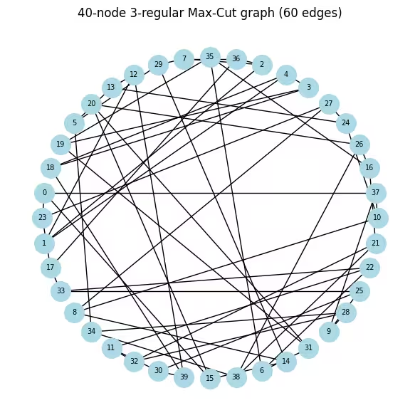
# A 3-regular graph (every node has exactly 3 neighbors) is a standard QAOA
N_LARGE = 40
G_large = nx.random_regular_graph(d=3, n=N_LARGE, seed=0)
edges_large = list(G_large.edges())
print(f"Graph: {N_LARGE} nodes, {len(edges_large)} edges (3-regular)")

# Visualize the graph so it is clear what problem we are solving before any
# quantum work. Nodes in a circular layout; each edge contributes +1 to the
# cut value when its endpoints land in different partitions.
pos_large = nx.circular_layout(G_large)
fig, ax = plt.subplots(figsize=(6, 6))
nx.draw(
    G_large,
    pos_large,
    with_labels=True,
    node_color="lightblue",
    node_size=400,
    font_size=7,
    ax=ax,
)
ax.set_title(f"40-node 3-regular Max-Cut graph ({len(edges_large)} edges)")
plt.tight_layout()
plt.show()

# Same Maxcut → OptimizationProblem → QUBO → Ising pipeline as the small example,
# applied to the 40-node graph.
prob_large = Maxcut(G_large).to_optimization_problem()
converter_large = OptimizationProblemToQubo()
qubo_large = converter_large.convert(prob_large)
cost_op_large, offset_large = to_ising(qubo_large)
n_qubits_large = cost_op_large.num_qubits
print(
    f"Cost operator: {n_qubits_large} qubits, {len(cost_op_large)} Pauli terms"
)

# ── Step 1b: QP relaxation (multi-start L-BFGS-B) ─────────────────────────
# Same multi-start approach as the small example. At 40 qubits the relaxed
# landscape has many more local minima, so 200 random starts are essential
# to find a low-energy warm-start point.
Q_large = qubo_large.objective.quadratic.to_array(symmetric=True)
mu_large = qubo_large.objective.linear.to_array()

def qp_obj_large(x):
    return x @ Q_large @ x + mu_large @ x + qubo_large.objective.constant

bounds_large = [(0.0, 1.0)] * n_qubits_large
rng_qp = np.random.default_rng(42)
best_val_large, c_star_large = np.inf, None

for _ in range(200):
    x0 = rng_qp.uniform(0.0, 1.0, n_qubits_large)
    res = minimize(qp_obj_large, x0, method="L-BFGS-B", bounds=bounds_large)
    if res.fun < best_val_large:
        best_val_large, c_star_large = res.fun, res.x

# Regularize and convert to rotation angles (same formula as small example)
epsilon_large = 0.25
c_clipped_large = np.clip(c_star_large, epsilon_large, 1 - epsilon_large)
thetas_large = 2 * np.arcsin(np.sqrt(c_clipped_large))
print(
    f"c* range: [{c_star_large.min():.3f}, {c_star_large.max():.3f}]  "
    f"theta range: [{thetas_large.min():.3f}, {thetas_large.max():.3f}] rad"
)

# Plot the distribution of c* values to see how much structure the relaxation
# extracted. Values near 0/1 mean confident assignments; values near 0.5 mean
# the classical solver was uncertain and quantum exploration is most needed there.
fig, ax = plt.subplots(figsize=(6, 3))
ax.hist(c_star_large, bins=20, color="steelblue", edgecolor="white")
ax.axvline(0.5, color="k", linestyle="--", label="Uniform prior (std QAOA)")
ax.set_xlabel(r"$c^*_i$")
ax.set_ylabel("Count")
ax.set_title(r"Distribution of warm-start values $c^*_i$ (40-node graph)")
ax.legend()
plt.tight_layout()
plt.show()

# ── Step 1c: Build WS-QAOA circuit ─────────────────────────────────────────
# Reuse build_ws_qaoa from the small-scale section unchanged; the helper
# scales automatically with n_qubits and the cost operator size.
p_large = 1
ws_qc_large, ws_gammas_large, ws_betas_large = build_ws_qaoa(
    cost_op_large, p_large, n_qubits_large, thetas_large
)
ws_qc_large.measure_all()

# ── Step 2: Transpile to hardware-native gates ──────────────────────────
# generate_preset_pass_manager compiles the abstract circuit to th
# gate set of the backend and inserts SWAP gates wherever the cost Hamiltonian
# couples qubits that are not directly connected on the processor.
pm = generate_preset_pass_manager(optimization_level=3, backend=backend)
ws_isa_large = pm.run(ws_qc_large)

ecr_count = ws_isa_large.count_ops().get("ecr", 0)
print(
    f"\nTranspiled circuit: 2Q depth={ws_isa_large.depth(lambda x: x.operation.num_qubits == 2)}"
)
ws_isa_large.draw("mpl", fold=-1)

Graph: 40 nodes, 60 edges (3-regular)

Cost operator: 40 qubits, 60 Pauli terms
c* range: [0.000, 1.000]  theta range: [1.047, 2.094] rad

Transpiled circuit: 2Q depth=86

# ── Classical baseline via simulated annealing ────────────────────
# Run SA before any hardware calls to get a strong classical reference cut
# value. SA is fast (seconds), needs no solver license, and reliably finds
# near-optimal solutions on 40-node graphs. We use sa_cut as the denominator
# for the approximation ratio instead of the looser QP upper bound.
#
# At each step we flip a random node and accept the move if it improves the
# cut, or with probability exp(delta/T) otherwise. Temperature T decays
# geometrically, allowing uphill moves early on to escape local minima.
def simulated_annealing_maxcut(
    G, seed=0, T0=2.0, T_min=1e-4, alpha=0.995, n_steps=100_000
):
    rng_sa = np.random.default_rng(seed)
    n = G.number_of_nodes()
    x = rng_sa.integers(0, 2, n)
    best_x = x.copy()
    best_cut = sum(1 for u, v in G.edges() if x[u] != x[v])
    T = T0
    for _ in range(n_steps):
        i = rng_sa.integers(0, n)
        delta = sum((-1 if x[i] != x[nb] else 1) for nb in G.neighbors(i))
        if delta > 0 or rng_sa.random() < np.exp(delta / T):
            x[i] ^= 1
            cut = sum(1 for u, v in G.edges() if x[u] != x[v])
            if cut > best_cut:
                best_cut, best_x = cut, x.copy()
        T = max(T * alpha, T_min)
    return best_x, best_cut

sa_solution, sa_cut = simulated_annealing_maxcut(G_large)
print(f"Simulated annealing cut value: {sa_cut}  (classical reference)")

# ── Step 3: Execution on hardware ───────────────────────────
# A Session reserves the backend so the COBYLA iterations and final sampling
# run back-to-back without re-queuing between jobs — important when the
# optimizer submits many short jobs sequentially. All jobs are tagged with
# "TUT_WSQAOA" for traceability in the IBM Quantum dashboard.
#
# EstimatorV2 with resilience_level=1 enables twirled readout error extinction
# (TREX), which corrects systematic measurement bit-flip errors without extra
# circuit overhead. 4096 shots per call balances estimation noise vs. job time.
estimator_options = EstimatorOptions()
estimator_options.resilience_level = 1
estimator_options.default_shots = 4096
estimator_options.environment.job_tags = ["TUT_WSQAOA"]

# Align the cost observable with the physical qubit layout chosen by the transpiler
cost_op_isa = cost_op_large.apply_layout(ws_isa_large.layout)
ws_param_order_isa = list(ws_isa_large.parameters)

ws_history_hw = []

with Session(backend=backend) as session:
    estimator_hw = Estimator(mode=session, options=estimator_options)

    def hw_cost_fn(params):
        bound = ws_isa_large.assign_parameters(
            dict(zip(ws_param_order_isa, params))
        )
        energy = (
            estimator_hw.run([(bound, cost_op_isa)]).result()[0].data.evs.real
        )
        ws_history_hw.append(float(energy))
        print(
            f"  iter {len(ws_history_hw):>3d}  <H_C> = {energy:.4f}", end="\r"
        )
        return float(energy)

    # Warm-start initialization: gamma=0 means the cost unitary is the identity on
    # the first call, so COBYLA immediately evaluates the warm-start state itself —
    # a much better starting signal than a random point.
    ws_params0_hw = np.concatenate(
        [np.zeros(p_large), np.full(p_large, np.pi / 4)]
    )

    ws_result_hw = minimize(
        hw_cost_fn,
        ws_params0_hw,
        method="COBYLA",
        options={"maxiter": 150, "rhobeg": 0.3},
    )
    print(
        f"\nOptimization complete: energy={ws_result_hw.fun:.4f}, "
        f"iterations={len(ws_history_hw)}"
    )

    # ── Step 3b: Sample the optimized circuit ──────────────────────────────────
    # Use 8192 shots for the final sample to get a reliable mode estimate.
    sampler_hw = Sampler(
        mode=session,
        options={"environment": {"job_tags": ["TUT_WSQAOA"]}},
    )
    ws_bound_hw = ws_isa_large.assign_parameters(
        dict(zip(ws_param_order_isa, ws_result_hw.x))
    )
    counts_hw = (
        sampler_hw.run([ws_bound_hw], shots=8192)
        .result()[0]
        .data.meas.get_counts()
    )

best_bs_hw = max(counts_hw, key=counts_hw.get)
best_count = counts_hw[best_bs_hw]
total_shots = sum(counts_hw.values())

# Decode: Qiskit returns bitstrings with qubit 0 at the rightmost position,
# so reversing the string maps character index i to variable x_i.
cut_val_hw, s0_hw, s1_hw = evaluate_cut(best_bs_hw[::-1], G_large)

# Compare against simulated annealing.
# A ratio >= 1.0 means WS-QAOA matched or beat the classical SA solution.
# A ratio close to 1.0 (e.g. > 0.95) shows the quantum result is competitive.
approx_ratio_hw = cut_val_hw / sa_cut
print(
    f"Most-probable bitstring frequency: {best_count}/{total_shots} "
    f"({100*best_count/total_shots:.1f}%)"
)
print(
    f"WS-QAOA cut: {cut_val_hw}  |  SA cut: {sa_cut}  "
    f"|  Approximation ratio vs SA: {approx_ratio_hw:.4f}"
)

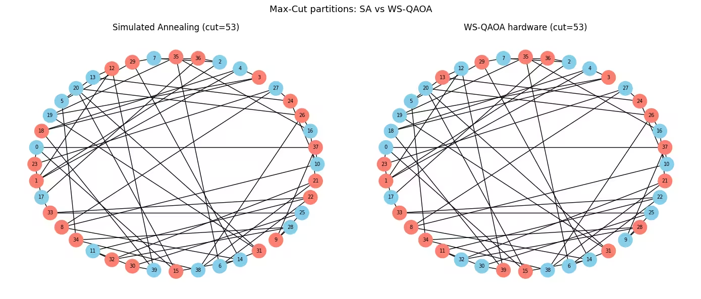
# Visualize both solutions side-by-side on the graph.
# Blue = partition S, orange = partition S-bar.
# Edges crossing between colors are the ones counted in the cut.
fig, axes = plt.subplots(1, 2, figsize=(14, 6))
for ax, assignment, cut, title in [
    (
        axes[0],
        list(sa_solution),
        sa_cut,
        f"Simulated Annealing (cut={sa_cut})",
    ),
    (
        axes[1],
        [int(b) for b in best_bs_hw[::-1]],
        cut_val_hw,
        f"WS-QAOA hardware (cut={cut_val_hw})",
    ),
]:
    colors = [
        "skyblue" if assignment[i] == 0 else "salmon" for i in G_large.nodes()
    ]
    nx.draw(
        G_large,
        pos_large,
        with_labels=True,
        node_color=colors,
        node_size=400,
        font_size=7,
        ax=ax,
    )
    ax.set_title(title)
plt.suptitle("Max-Cut partitions: SA vs WS-QAOA", fontsize=13)
plt.tight_layout()
plt.show()

# ── Step 4: Convergence plot and summary ──────────────────────────────────
# On real hardware the trace will be noisy (shot noise + gate errors), but the
# overall downward trend confirms that COBYLA is making progress despite noise.
fig, ax = plt.subplots(figsize=(7, 4))
ax.plot(ws_history_hw, color="tab:orange", label="WS-QAOA (hardware)")
ax.axhline(
    ws_result_hw.fun,
    color="tab:orange",
    linestyle=":",
    label=f"Final energy ({ws_result_hw.fun:.3f})",
)
ax.set_xlabel("Optimizer call")
ax.set_ylabel(r"$\langle H_C \rangle$")
ax.set_title(f"WS-QAOA convergence on {backend.name} (40 qubits, p=1)")
ax.legend()
plt.tight_layout()
plt.show()

print("\n=== Large Scale Summary ===")
print(f"{'Metric':<38} {'Value':>10}")
print("-" * 50)
print(f"{'Nodes / Edges':<38} {N_LARGE:>5} / {len(edges_large):<4}")
print(f"{'QAOA layers (p)':<38} {p_large:>10}")
print(f"{'Transpiled ECR gate count':<38} {ecr_count:>10}")
print(f"{'Transpiled circuit depth':<38} {ws_isa_large.depth():>10}")
print(f"{'Optimizer iterations':<38} {len(ws_history_hw):>10}")
print(f"{'WS-QAOA energy (hardware)':<38} {ws_result_hw.fun:>10.4f}")
print(f"{'Cut value':<38} {cut_val_hw:>10}")
print(f"{'Simulated annealing cut value':<38} {sa_cut:>10}")
print(f"{'Approximation ratio (vs SA)':<38} {approx_ratio_hw:>10.4f}")

Simulated annealing cut value: 53  (classical reference)
  iter  31  <H_C> = -12.4094
Optimization complete: energy=-13.0256, iterations=31
Most-probable bitstring frequency: 4/8192 (0.0%)
WS-QAOA cut: 53  |  SA cut: 53  |  Approximation ratio vs SA: 1.0000

=== Large Scale Summary ===
Metric                                      Value
--------------------------------------------------
Nodes / Edges                             40 / 60  
QAOA layers (p)                                 1
Transpiled ECR gate count                       0
Transpiled circuit depth                      276
Optimizer iterations                           31
WS-QAOA energy (hardware)                -13.0256
Cut value                                      53
Simulated annealing cut value                  53
Approximation ratio (vs SA)                1.0000

Nächste Schritte

Empfehlungen

Wenn du diese Arbeit interessant fandest, könnten dich folgende Materialien interessieren:

• Höhere QAOA-Schichten: Erhöhe p, um zu sehen, wie sich beide Algorithmen mit mehr Schaltkreisschichten verbessern und ob der WS-QAOA-Vorteil bei geringer Tiefe bestehen bleibt.
• Qiskit-Addon-Optimierungs-Mapper: Sieh dir die Dokumentation an und versuche, verschiedene kombinatorische Probleme zu modellieren oder unterschiedliche Solver für die kontinuierliche Relaxation zu verwenden.

Referenzen

[1] D. J. Egger, J. Mareček, and S. Woerner, "Warm-starting quantum optimization," Quantum, vol. 5, p. 479, 2021. arXiv:2009.10095

[2] E. Farhi, J. Goldstone, and S. Gutmann, "A quantum approximate optimization algorithm," arXiv:1411.4028, 2014.