Einsetzen der Ergodizität über Skalen hinweg
Dieses Notebook führt durch die Ausführung und Analyse der Experimente in Onset of Ergodicity Across Scales on a Digital Quantum Processor [arXiv:2603.12236]: vom Modell zu den Circuits, von Bitstrings zu Entropien, von verrauschten Daten zu mitigierten Ergebnissen und von einer 16-Qubit-Simulation zu einem 64-Qubit-Lauf auf einem IBM Quantum® Nighthawk-Prozessor. Der gesamte Code steht hier, und jede Funktion wird dort definiert, wo sie zuerst gebraucht wird.
| Zeit | Abschnitt |
|---|---|
| 0–1 Min. | Einrichtung |
| 1–6 Min. | 1. Vom Modell zu einem Circuit |
| 6–12 Min. | 2. Was zu messen ist und wie man es schätzt |
| 12–19 Min. | 3. Rauschen und wie man es rückgängig macht |
| 19–24 Min. | 4. Lauf im großen Maßstab |
| 24–33 Min. | 5. Die Hardwaredaten |
| 33–35 Min. | Abschluss |
Zum Mitmachen. Führe die Zellen von oben nach unten aus. Ein IBM Quantum-Konto ist nicht nötig; die Zellen, die Hardware-Jobs übergeben, sind abgeschaltet, und Abschnitt 5 analysiert einen gespeicherten Hardware-Lauf, den die Einrichtungszelle nach data/ herunterlädt. Diskussionsfragen sind mit Question markiert; versuche zu antworten, bevor du die Antwort öffnest.
Einrichtung
Erfordert Python 3.12 oder neuer und die folgenden Pakete:
-
Qiskit SDK v2.5 oder neuer, mit Unterstützung für Visualisierung
-
Qiskit Runtime v0.49 oder neuer (
pip install qiskit-ibm-runtime) -
Qiskit Aer v0.17 oder neuer (
pip install qiskit-aer) -
Samplomatic v0.21 oder neuer (
pip install samplomatic) -
NumPy und Matplotlib
Die Einrichtungszelle lädt außerdem den gespeicherten Hardware-Lauf und die MPS-Referenzen (etwa 9 MB) nach data/ herunter, sofern sie nicht bereits dort liegen.
# Added by doQumentation — installs the packages this notebook needs if they are missing
import importlib.util

_needed = {"matplotlib": "matplotlib", "numpy": "numpy", "qiskit": "qiskit", "qiskit_aer": "qiskit-aer", "qiskit_ibm_runtime": "qiskit-ibm-runtime", "samplomatic": "samplomatic"}
_missing = [pip for module, pip in _needed.items()
            if importlib.util.find_spec(module) is None]
# One at a time, so a package that fails to install does not block the others
for _pip in _missing:
    %pip install -q {_pip}
if not _missing:
    print("\u2713 All required packages are installed")
from math import comb
from pathlib import Path
from urllib.request import urlretrieve

import matplotlib.pyplot as plt
import numpy as np
from qiskit import ClassicalRegister, QuantumCircuit, QuantumRegister
from qiskit.primitives import StatevectorSampler
from qiskit.quantum_info import (
    PauliLindbladMap,
    QubitSparsePauli,
    Statevector,
)
from qiskit.transpiler import generate_preset_pass_manager
from qiskit_aer import AerSimulator
from qiskit_aer.noise import NoiseModel, ReadoutError, depolarizing_error
from qiskit_aer.primitives import SamplerV2 as AerSampler

RUN_ON_HARDWARE = (
    False  # True submits the 8x8 jobs in section 4 (needs Nighthawk access)
)
COMPUTE_MPS_REFERENCES = False  # True recomputes the MPS references in section 5 (about 18 minutes)

# Download the saved hardware run and MPS references, unless they are already in data/
data_url = "https://raw.githubusercontent.com/Qiskit/documentation/main/datasets/tutorials/onset-of-ergodicity"
Path("data").mkdir(exist_ok=True)
for name in ("hardware_run.npz", "mps_references_all.npz"):
    if not Path("data", name).exists():
        urlretrieve(f"{data_url}/{name}", Path("data", name))
1. Vom Modell zu einem Circuit
Das Zwei-Qubit-Gate
Jede Bindung des Gitters erhält dasselbe Zwei-Qubit-Gate, bestehend aus einem Heisenberg-Verschränker, gefolgt von zufälligen Feldern:
wobei für jedes Gate gleichverteilt aus gezogen wird.
Question. Wie würdest du in Gates zerlegen, die die Hardware ausführen kann?
Antwort
Die Felder sind einfach. ist eine Ein-Qubit-Rotation auf jedem Qubit.
Der Verschränker ist der schwierige Teil. , und kommutieren, daher zerfällt er in drei Rotationen, , und . Jede braucht zwei CNOTs, was sechs CNOTs pro Gate ergibt.
Es gibt einen besseren Weg. Jedes Zwei-Qubit-Gate lässt sich aus höchstens drei CNOTs und Ein-Qubit-Rotationen bauen. Der optimale Circuit geht von der Form aus, und dieser Verschränker hat diese Form bereits mit . Er lässt sich also direkt auf drei CNOTs abbilden, und die Ein-Qubit-Winkel sind linear in . Der Experimentcode baut das Gate auf diese Weise.
Auf Hardware fügt jedes Zwei-Qubit-Gate Rauschen hinzu, daher ist es wichtig, die Anzahl der CNOTs zu halbieren.
def xxyyzz_gate(circuit, coupling, i, j):
    # exp(iJ(XX + YY + ZZ)) with three CNOTs; only the rotation angles depend on J
    circuit.rz(-np.pi / 2, j)
    circuit.cx(j, i)
    circuit.rz(np.pi / 2 - 2 * coupling, i)
    circuit.ry(2 * coupling - np.pi / 2, j)
    circuit.cx(i, j)
    circuit.ry(np.pi / 2 - 2 * coupling, j)
    circuit.cx(j, i)
    circuit.rz(np.pi / 2, i)

def heisenberg_gate(circuit, coupling, i, j, h_i, h_j):
    # The entangler first, then the random fields exp(i h Z)
    xxyyzz_gate(circuit, coupling, i, j)
    circuit.rz(-2 * h_i, i)
    circuit.rz(-2 * h_j, j)

h_i, h_j = 0.3, -0.7
gate = QuantumCircuit(2)
heisenberg_gate(gate, 0.05 * np.pi, 0, 1, h_i, h_j)
gate.draw("mpl")

Das Backsteinmuster und der Floquet-Zyklus
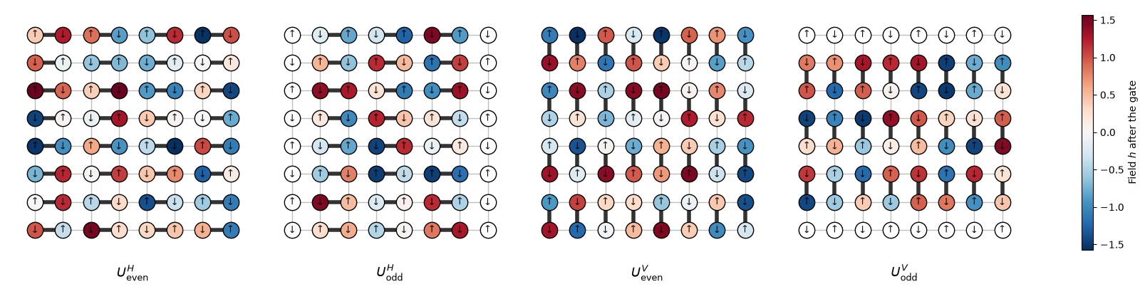
Die Gates überdecken das Quadratgitter in vier Subschichten nicht überlappender Bindungen, einem Backsteinmuster: horizontale Bindungen, die in geraden Spalten beginnen, dann in ungeraden Spalten, dann vertikale Bindungen, die in geraden Zeilen beginnen, dann in ungeraden Zeilen. Qubit sitzt am Gitterplatz .
def brickwork_layers(num_cols, num_rows):
    # Bonds of the square lattice, in the four sublayers of the brickwork
    def qubit(x, y):
        return y * num_cols + x

    layers = []
    for p in (0, 1):  # horizontal bonds starting on even, then odd, columns
        layers.append(
            [
                (qubit(x, y), qubit(x + 1, y))
                for y in range(num_rows)
                for x in range(p, num_cols - 1, 2)
            ]
        )
    for p in (0, 1):  # vertical bonds starting on even, then odd, rows
        layers.append(
            [
                (qubit(x, y), qubit(x, y + 1))
                for y in range(p, num_rows - 1, 2)
                for x in range(num_cols)
            ]
        )
    return layers

brickwork_layers(4, 4)
[[(0, 1), (2, 3), (4, 5), (6, 7), (8, 9), (10, 11), (12, 13), (14, 15)],
 [(1, 2), (5, 6), (9, 10), (13, 14)],
 [(0, 4), (1, 5), (2, 6), (3, 7), (8, 12), (9, 13), (10, 14), (11, 15)],
 [(4, 8), (5, 9), (6, 10), (7, 11)]]
Die vier Subschichten bilden einen Floquet-Zyklus. Der Zyklus wiederholt sich -mal mit denselben Feldern, sodass die Dynamik im Raum zufällig und in der Zeit periodisch ist. Der Circuit beginnt im Néel-Zustand, und ist die halbe Seitenlänge des Gitters. Die nächste Zelle zeichnet einen Floquet-Zyklus des -Hardwaregitters, Subschicht für Subschicht, mit den Feldern des Hardware-Laufs, im Stil von Abbildung 5 der Veröffentlichung. Dicke Bindungen sind die Gates jeder Subschicht. Jedes Qubit, auf das ein Gate wirkt, wird nach dem zufälligen Feld eingefärbt, das es anschließend erhält, und untätige Qubits sind weiß. Die Pfeile zeigen den Néel-Anfangszustand, mit für . In der Abbildung der Veröffentlichung werden die vertikalen Subschichten zuerst angewendet; keine der beiden Reihenfolgen dürfte die Physik verändern.
# circuit structure, 8x8 system:
side = 8
all_bonds = [bond for layer in brickwork_layers(side, side) for bond in layer]

# get the disorder parameters for a given system:
def sample_disorder(num_cols, num_rows, rng):
    # One pair of fields (h_i, h_j) per gate, reused in every Floquet cycle
    return [
        [
            (bond, tuple(rng.uniform(-np.pi / 2, np.pi / 2, 2)))
            for bond in layer
        ]
        for layer in brickwork_layers(num_cols, num_rows)
    ]

# build the structure for the 8x8 system
example_disorder = sample_disorder(
    side, side, np.random.default_rng(7)
)  # the hardware fields (section 4)
titles = [
    r"$U^H_\mathrm{even}$",
    r"$U^H_\mathrm{odd}$",
    r"$U^V_\mathrm{even}$",
    r"$U^V_\mathrm{odd}$",
]
norm = plt.Normalize(-np.pi / 2, np.pi / 2)
cmap = plt.get_cmap("RdBu_r")

fig, axes = plt.subplots(1, 4, figsize=(16, 4.8), layout="constrained")
for ax, title, sublayer in zip(axes, titles, example_disorder):
    for i, j in all_bonds:
        ax.plot(
            [i % side, j % side],
            [i // side, j // side],
            color="0.75",
            lw=1,
            zorder=0,
        )
    fields = {}
    for (i, j), (h_i, h_j) in sublayer:
        ax.plot(
            [i % side, j % side],
            [i // side, j // side],
            color="0.2",
            lw=4,
            zorder=1,
        )
        fields[i], fields[j] = h_i, h_j
    for q in range(side * side):
        x, y = q % side, q // side
        ax.scatter(
            x,
            y,
            s=260,
            color=cmap(norm(fields[q])) if q in fields else "white",
            edgecolor="black",
            zorder=2,
        )
        ax.text(
            x,
            y,
            "↓" if (x + y) % 2 else "↑",
            ha="center",
            va="center",
            fontsize=9,
            zorder=3,
        )
    ax.set_aspect("equal")
    ax.set_xlim(-1, side)  # padding, so the panels read as separate steps
    ax.set_ylim(side, -1)
    ax.axis("off")
    ax.set_title(title, y=-0.1, fontsize=13)
fig.colorbar(
    plt.cm.ScalarMappable(norm=norm, cmap=cmap),
    ax=axes,
    shrink=0.7,
    label="Field $h$ after the gate",
)
plt.show()
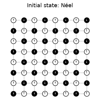
Definiere den Anfangszustand.
# initial state
def neel_state(circuit, num_cols, num_rows, layout):
    for y in range(num_rows):
        for x in range(num_cols):
            if (x + y) % 2 == 1:
                circuit.x(layout[y * num_cols + x])
# The initial Néel state: |1⟩ (black, ↓) on odd sites, |0⟩ (white, ↑) on even sites

fig, ax = plt.subplots(figsize=(4, 4.4))
for i, j in all_bonds:
    ax.plot(
        [i % side, j % side],
        [i // side, j // side],
        color="0.75",
        lw=1,
        zorder=0,
    )
for q in range(side * side):
    x, y = q % side, q // side
    excited = (x + y) % 2 == 1
    ax.scatter(
        x,
        y,
        s=150,
        color="black" if excited else "white",
        edgecolor="black",
        zorder=2,
    )
    ax.text(
        x,
        y,
        "↓" if excited else "↑",
        ha="center",
        va="center",
        fontsize=7,
        color="white" if excited else "black",
        zorder=3,
    )
ax.set_aspect("equal")
ax.set_xlim(-1, side)
ax.set_ylim(side, -1)
ax.axis("off")
ax.set_title("Initial state: Néel", fontsize=13)
plt.show()
# actual circuit construction:
def heisenberg_floquet_circuit(
    num_cols, num_rows, coupling, num_cycles, disorder, measure=True
):
    num_qubits = num_cols * num_rows
    circuit = QuantumCircuit(num_qubits)
    neel_state(circuit, num_cols, num_rows, list(range(num_qubits)))
    cycle = QuantumCircuit(num_qubits)
    for sublayer in disorder:
        for (i, j), (h_i, h_j) in sublayer:
            heisenberg_gate(cycle, coupling, i, j, h_i, h_j)
    for _ in range(num_cycles):
        circuit.compose(cycle, inplace=True)
    if measure:
        circuit.measure_all()
    return circuit
Ein -Beispiel
Die Simulationen verwenden ein -Gitter mit zwei Zyklen und die in der Veröffentlichung untersuchten Kopplungen . Ein Satz von Feldern wird für jede Kopplung wiederverwendet.
# simulation parameters:
num_cols = num_rows = 4
num_qubits = num_cols * num_rows
num_cycles = 2
couplings = (
    np.array([0.005, 0.01, 0.02, 0.03, 0.04, 0.05, 0.06, 0.08, 0.10, 0.125])
    * np.pi
)
disorder = sample_disorder(num_cols, num_rows, np.random.default_rng(42))

# circuit construction:
logical_circuits = [
    heisenberg_floquet_circuit(
        num_cols, num_rows, coupling, num_cycles, disorder
    )
    for coupling in couplings
]
logical_circuits[5].draw(output="mpl", fold=-1)

# transpiling the circuit:
pass_manager = generate_preset_pass_manager(
    optimization_level=3,
    basis_gates=["cz", "rz", "sx", "x"],
    seed_transpiler=7,
)
circuits = [pass_manager.run(circuit) for circuit in logical_circuits]

def two_qubit_stats(circuit):
    count = sum(1 for inst in circuit.data if inst.operation.num_qubits == 2)
    depth = circuit.depth(lambda inst: inst.operation.num_qubits == 2)
    return count, depth

stats = {two_qubit_stats(circuit) for circuit in circuits}
assert len(stats) == 1, "the CZ structure should not depend on J"
num_cz, depth = stats.pop()
print(
    f"{num_qubits} qubits: {num_cz} CZ gates in {depth} layers, for every coupling"
)
circuits[5].draw("mpl", fold=-1, scale=0.4)
16 qubits: 144 CZ gates in 24 layers, for every coupling

Ein cleverer Compiler ist nicht nötig, weil die Circuits (und das Experiment) für IBM Nighthawk entworfen wurden.
Das -Gitter simulieren
Für das -Gitter kannst du beides tun: den exakten Zustand bei jeder Kopplung berechnen und jeden Circuit mit 10.000 Shots sampeln, wie es ein Experiment täte. Die Shots werden mit der Form (Batches, Shots, Qubits) gespeichert, demselben Layout wie die Randomisierungen in den Hardwaredaten. Hier bilden alle 10.000 Shots einen einzigen Batch, sodass das Bootstrapping über Batches kein Shot-Rauschen hinzufügt und die Fehlerbalken im nächsten Diagramm nur die Streuung zwischen den Marginalpositionen zeigen.
exact_states = [
    Statevector(
        heisenberg_floquet_circuit(
            num_cols, num_rows, c, num_cycles, disorder, measure=False
        )
    )
    for c in couplings
]

shots = 10_000
results = (
    StatevectorSampler(default_shots=shots, seed=1234).run(circuits).result()
)

# the output of the simulation for the 10 couplings
bits = [
    result.data.meas.to_bool_array(order="little").reshape(
        1, 10_000, num_qubits
    )
    for result in results
]

print(bits[0])
[[[False  True False ... False  True False]
  [False  True False ... False  True False]
  [False  True False ... False  True False]
  ...
  [False  True False ... False  True False]
  [False  True False ... False  True False]
  [False  True False ... False  True False]]]
2. Was zu messen ist und wie man es schätzt
Die IPR und die Kollisionsentropie
Für eine Marginale aus Qubits mit Bitstring-Verteilung ist die zu schätzende Größe das inverse Partizipationsverhältnis (IPR) der Marginalverteilung und daraus die Kollisionsentropie:
ist auch die Wahrscheinlichkeit, dass zwei Shots bei der Marginale übereinstimmen. Ein Produktzustand hat , und ein Zufallszustand hat , sodass von 0 auf etwa Bit steigt, wenn die Marginale zufällig wird.
Schätzer 1: Paare von Shots zählen
Question. Wie schätzt du diese Größe aus deinen Shots?
Antwort
Der naive Schätzer berechnet jedes aus den Shots als und summiert dann . Dieser Schätzer ist verzerrt.
zählt jeden Shot als mit sich selbst übereinstimmend, was die Schätzung nach oben treibt: Im Mittel ergibt sie statt . Da die Wahrscheinlichkeit ist, dass zwei Shots übereinstimmen, zähle nur Paare verschiedener Shots:
Dieser ist unverzerrt, und genau ihn berechnet ipr_from_shots weiter unten.
# IPR expectation values:

# refactor this function cause it does not scale
def ipr_from_shots(bits):
    # Pair-counting estimate of the IPR of a marginal: the fraction of pairs of different shots
    # that agree on it. bits holds the marginal's qubits only, with shape (randomizations, shots,
    # qubits), and all randomizations are pooled.
    n = bits.shape[-1]
    outcomes = bits @ 2 ** np.arange(
        n
    )  # each shot's marginal bitstring, read as an integer
    counts = np.bincount(outcomes.ravel())  # how often each outcome occurs
    total = counts.sum()
    return float((counts * (counts - 1)).sum() / (total * (total - 1)))

def collision_entropy(ipr):
    return -np.log2(ipr)
Schätzer 2: Parseval-Entwicklung
Die IPR lässt sich auch über die Paritäten aller nichtleeren Teilmengen der Marginale schreiben:
Diese Form ist wichtig, weil Fehlermitigationsmethoden wie PEA auf Erwartungswerten arbeiten, nicht auf Wahrscheinlichkeiten. Ein Qubit: Die Ergebniswahrscheinlichkeiten sind und , also
Eine -Marginale: Wenn ihre Qubits mit bezeichnet sind, hat die Marginale Paritäten: 4 einzelne Qubits, 6 Paare, 4 Tripel und die gesamte Marginale, also
def parity_supports(patch):
    # All nonempty subsets S of the marginal
    return sorted(
        [
            tuple(q for k, q in enumerate(patch) if mask & (1 << k))
            for mask in range(1, 1 << len(patch))
        ],
        key=len,
    )

def parity_expectation_values(bits, supports):
    # Shot-averaged <Z_S> for every support, per randomization
    signs = 1 - 2 * bits.astype(np.int8)
    return np.stack(
        [signs[..., list(s)].prod(axis=-1).mean(axis=-1) for s in supports],
        axis=-1,
    )

# Example: the parities of a 3-qubit marginal made of lattice qubits 5, 6, and 9
print(parity_supports([5, 6, 9]))
print(f"A 3×3 marginal has {len(parity_supports(range(9)))} parities")
[(5,), (6,), (9,), (5, 6), (5, 9), (6, 9), (5, 6, 9)]
A 3×3 marginal has 511 parities
Mittelung über Marginalen
Weitere nützliche Funktionen: Haar-Werte, Auswahl von Marginalen, Bootstrapping und Mittelung.
# functions for the Haar values on plots:
def haar_ipr(num_patch, num_qubits):
    # Mean IPR of a marginal for Haar-random states in the sector with num_qubits // 2 ones
    weight = num_qubits // 2
    dimension = comb(num_qubits, weight)
    total = 0
    for k in range(num_patch + 1):  # k ones on the marginal
        rest = (
            comb(num_qubits - num_patch, weight - k) if weight - k >= 0 else 0
        )
        total += comb(num_patch, k) * rest * (rest + 1)
    return total / (dimension * (dimension + 1))

def haar_entropy(num_patch, num_qubits):
    return collision_entropy(haar_ipr(num_patch, num_qubits))

# definitions of positions in the lattice:
def patch_qubits(anchor, shape, num_cols):
    # Lattice indices of a rectangular marginal with its top-left corner at anchor
    (x0, y0), (width, height) = anchor, shape
    return [
        (y0 + dy) * num_cols + (x0 + dx)
        for dy in range(height)
        for dx in range(width)
    ]

def all_positions(shape, num_cols, num_rows):
    # Every placement of a (width, height) marginal on the lattice
    width, height = shape
    return [
        patch_qubits((x, y), shape, num_cols)
        for y in range(num_rows - height + 1)
        for x in range(num_cols - width + 1)
    ]

# bootstrapping for error bars:
bootstrap_rng = np.random.default_rng(0)

def bootstrap_error(statistic, *samples, axis=0, num_resamples=50):
    # Shot noise of a statistic, from resampling the randomizations (along axis of every
    # sample) with replacement
    values = []
    for _ in range(num_resamples):
        resampled = [
            np.take(
                x,
                bootstrap_rng.integers(0, x.shape[axis], x.shape[axis]),
                axis=axis,
            )
            for x in samples
        ]
        values.append(statistic(*resampled))
    return float(np.std(values, ddof=1))

# averaging the ipr over marginals:
def average_ipr(iprs, shot_errors):
    # iprs and shot_errors have shape (positions, couplings). The mean IPR over positions, and its
    # error: the spread between positions plus the shot noise of each (law of total variance)
    iprs, shot_errors = np.asarray(iprs), np.asarray(shot_errors)
    count = len(iprs)
    variance = (
        iprs.var(axis=0, ddof=1) / count
        + (shot_errors**2).sum(axis=0) / count**2
    )
    return iprs.mean(axis=0), np.sqrt(variance)
# Calculating exact simulation entropies:
patch_shapes = {
    "1×1": (1, 1),
    "1×2": (2, 1),
    "2×2": (2, 2),
    "2×3": (3, 2),
    "3×3": (3, 3),
}

# calculate the exact entropies:
sim_positions = {
    label: all_positions(shape, num_cols, num_rows)
    for label, shape in patch_shapes.items()
}
exact_iprs = {  # shape (positions, couplings)
    label: np.array(
        [
            [(s.probabilities(qargs=q) ** 2).sum() for s in exact_states]
            for q in qubit_lists
        ]
    )
    for label, qubit_lists in sim_positions.items()
}
exact_entropies = {
    label: collision_entropy(v.mean(axis=0))
    for label, v in exact_iprs.items()
}

# Average IPR of every shape over its positions, from the sampled shots, then the entropy
iprs_from_shots = {}  # per shape: average IPR and its error, at every coupling
entropies_from_shots = {}  # per shape: average entropy and its error, at every coupling
for label, qubit_lists in sim_positions.items():
    iprs = [[ipr_from_shots(b[:, :, q]) for b in bits] for q in qubit_lists]

    # bootstrapping over subsampling for error bars:
    errors = [
        [bootstrap_error(ipr_from_shots, b[:, :, q]) for b in bits]
        for q in qubit_lists
    ]
    ipr, ipr_error = average_ipr(iprs, errors)
    iprs_from_shots[label] = (ipr, ipr_error)
    entropies_from_shots[label] = (
        collision_entropy(ipr),
        ipr_error / (ipr * np.log(2)),
    )
# Now plot the average IPR on the left, and the same averages as entropies on the right
colors = plt.cm.plasma(np.linspace(0.05, 0.8, len(patch_shapes)))
fig, (ax_ipr, ax_entropy) = plt.subplots(1, 2, figsize=(12.8, 4.2))
for (label, qubit_lists), color in zip(sim_positions.items(), colors):
    n = len(qubit_lists[0])
    ipr, ipr_error = iprs_from_shots[label]
    entropy, entropy_error = entropies_from_shots[label]
    # Left: the average IPR, with its exact value and its random-state value
    ax_ipr.axhline(haar_ipr(n, num_qubits), color=color, ls="dashdot", lw=0.9)
    ax_ipr.plot(
        couplings / np.pi, exact_iprs[label].mean(axis=0), color=color
    )
    ax_ipr.errorbar(
        couplings / np.pi,
        ipr,
        yerr=ipr_error,
        fmt="o",
        color=color,
        mec="white",
        ms=7,
        capsize=3,
        label=f"{label} ({len(qubit_lists)} positions)",
    )
    # Right: the average collision entropy
    ax_entropy.axhline(
        haar_entropy(n, num_qubits), color=color, ls="dashdot", lw=0.9
    )
    ax_entropy.plot(couplings / np.pi, exact_entropies[label], color=color)
    ax_entropy.errorbar(
        couplings / np.pi,
        entropy,
        yerr=entropy_error,
        fmt="o",
        color=color,
        mec="white",
        ms=7,
        capsize=3,
        label=f"{label} ({len(qubit_lists)} positions)",
    )
ax_ipr.set_yscale("log")
ax_ipr.set_ylabel("Average IPR")
ax_entropy.set_ylabel("Average collision entropy (bits)")
for ax in (ax_ipr, ax_entropy):
    ax.set_xlabel("Coupling $J/\\pi$")
fig.suptitle("Exact (lines) and sampled (dots), 4×4 lattice, 2 cycles")
ax_entropy.legend(title="Marginal", loc="upper left")
fig.tight_layout()
plt.show()
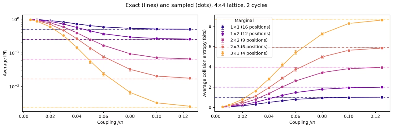
Jede Marginalverteilung steigt gleichmäßig auf ihren Wert für einen Zufallszustand an, und größere Marginalverteilungen erreichen ihn bei größeren .
3. Rauschen und wie man es rückgängig macht
Eine verrauschte Simulation
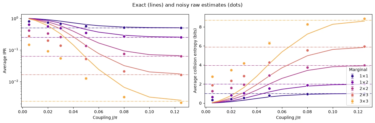
Füge nun Rauschen hinzu: 1 % depolarisierendes Zwei-Qubit-Rauschen auf jedem CZ-Gate und einen Auslesefehler von 3 % auf jedem Qubit, gesampelt mit dem Qiskit-Aer-Sampler. Mit 144 CZ-Gates im Circuit ist das deutlich weniger Rauschen als in den 8×8-Hardware-Circuits, aber genug, um die Wirkung zu sehen. Die Simulation verwendet sechs Kopplungen mit je 4.000 Shots und dauert etwa 1,5 Minuten.
Frage. Bevor du sie ausführst: Wird das System durch Rauschen stärker oder weniger stark thermalisiert aussehen?
Antwort
Stärker. Rauschen verwischt die Ergebnisse und treibt jede Marginalverteilung in Richtung Gleichverteilung, sodass der rohe IPR sinkt und die Entropie steigt. Ohne Fehlerminderung sieht Rauschen wie eine Thermalisierung aus, die gar nicht vorhanden ist, und die Übergänge treten zu früh auf.
# define the noise model

noise_model = NoiseModel()
# two qubit depolarizing noise:
noise_model.add_all_qubit_quantum_error(depolarizing_error(0.01, 2), ["cz"])
# symmetric readout noise:
noise_model.add_all_qubit_readout_error(
    ReadoutError([[0.97, 0.03], [0.03, 0.97]])
)

# simulation is done using trajectories
noisy_sampler = AerSampler(
    default_shots=4000,
    seed=1,
    options={"backend_options": {"noise_model": noise_model}},
)

# choose a subset of J values for speed:
noisy_indices = [
    0,
    2,
    3,
    5,
    7,
    9,
]  # J/π = 0.005, 0.02, 0.03, 0.05, 0.08, 0.125
noisy_results = noisy_sampler.run(
    [circuits[k] for k in noisy_indices]
).result()

# No twirling here, so the 20 "randomizations" are just batches of 200 shots
noisy_bits = {
    k: result.data.meas.to_bool_array(order="little").reshape(
        20, 200, num_qubits
    )
    for k, result in zip(noisy_indices, noisy_results)
}
# Calculating noisy entropies

# Average IPR of every shape over its positions, from the noisy shots, then the entropy
noisy_iprs = {}  # per shape: average IPR and its error, at every noisy coupling
noisy_entropies = {}  # per shape: average entropy and its error, at every noisy coupling
for label, qubit_lists in sim_positions.items():
    iprs = [
        [ipr_from_shots(noisy_bits[k][:, :, q]) for k in noisy_indices]
        for q in qubit_lists
    ]

    # bootstrapping over subsampling for error bars:
    errors = [
        [
            bootstrap_error(ipr_from_shots, noisy_bits[k][:, :, q])
            for k in noisy_indices
        ]
        for q in qubit_lists
    ]
    ipr, ipr_error = average_ipr(iprs, errors)
    noisy_iprs[label] = (ipr, ipr_error)
    noisy_entropies[label] = (
        collision_entropy(ipr),
        ipr_error / (ipr * np.log(2)),
    )
fig, (ax_ipr, ax_entropy) = plt.subplots(1, 2, figsize=(12.8, 4.2))
for (label, qubit_lists), color in zip(sim_positions.items(), colors):
    n = len(qubit_lists[0])
    ipr, ipr_error = noisy_iprs[label]
    entropy, entropy_error = noisy_entropies[label]
    # Left: the average IPR, with its exact value and its random-state value
    ax_ipr.axhline(haar_ipr(n, num_qubits), color=color, ls="dashdot", lw=0.9)
    ax_ipr.plot(
        couplings / np.pi, exact_iprs[label].mean(axis=0), color=color
    )
    ax_ipr.errorbar(
        couplings[noisy_indices] / np.pi,
        ipr,
        yerr=ipr_error,
        fmt="o",
        color=color,
        mec="white",
        ms=7,
        capsize=3,
        label=label,
    )
    # Right: the same averages as entropies
    ax_entropy.axhline(
        haar_entropy(n, num_qubits), color=color, ls="dashdot", lw=0.9
    )
    ax_entropy.plot(couplings / np.pi, exact_entropies[label], color=color)
    ax_entropy.errorbar(
        couplings[noisy_indices] / np.pi,
        entropy,
        yerr=entropy_error,
        fmt="o",
        color=color,
        mec="white",
        ms=7,
        capsize=3,
        label=label,
    )
ax_ipr.set_yscale("log")
ax_ipr.set_ylabel("Average IPR")
ax_entropy.set_ylabel("Average collision entropy (bits)")
for ax in (ax_ipr, ax_entropy):
    ax.set_xlabel("Coupling $J/\\pi$")
fig.suptitle("Exact (lines) and noisy raw estimates (dots)")
ax_entropy.legend(title="Marginal", loc="lower right")
fig.tight_layout()
plt.show()
Brainstorming: Wie würdest du das rückgängig machen?
Lösungsvorschlag
Bei kleinem ist der Zustand kaum verschränkt, daher lässt sich die ideale Antwort dort klassisch günstig berechnen, selbst für 64 Qubits. Das legt nahe, die Wirkung des Rauschens bei einer kleinen Kalibrierkopplung zu messen und damit jede andere Kopplung zu korrigieren. Dafür gibt es zwei naheliegende Wege, die Low-Entanglement-Kalibrierung (LEC) genannt werden:
LEC auf dem IPR. Skaliere den Überschuss des IPR gegenüber seinem Wert für eine Gleichverteilung, , mit einem Faktor pro Marginalverteilung:
LEC auf den -Erwartungswerten. Skaliere jede Parität der Marginalverteilung mit ihrem eigenen Faktor und rekonstruiere den IPR mit der Parseval-Formel:
Im Code wird jede quadrierte, skalierte Parität bereinigt, indem ihre Varianz subtrahiert wird, wie in Abschnitt 2.
Beide sind gleich, wenn jedes gleich ist.
Question. What are the pros and cons of these methods?
Antwort
Pros
-
Günstig: Vom Gerät sind keine zusätzlichen Daten nötig, nur eine klassische Simulation bei .
-
Nutzt die Struktur des Circuits: Die Circuit-Tiefe und die CZ-Layer ändern sich nicht mit , daher ist das Rauschen bei dasselbe Rauschen wie bei jedem anderen .
Cons
- Setzt voraus, dass die Wirkung des Rauschens auf die Observablen nicht von abhängt: Das Rauschen selbst ist gleich, aber wie es den IPR oder jedes dämpft, kann sich mit wachsendem ändern.
Beide Methoden an der verrauschten Simulation
# function to mitigate the IPR signal:
def mitigate_ipr_w_lec(
    ipr_raw, ipr_raw_calibration, ipr_ideal_calibration, num_patch
):
    # LEC on the IPR: one factor R0 for the excess over the uniform value
    uniform = 2.0**-num_patch
    factor = (ipr_ideal_calibration - uniform) / (
        ipr_raw_calibration - uniform
    )
    return uniform + factor * (ipr_raw - uniform)

# function used to calculate the target <Z> expectation values
def parities_from_probabilities(probabilities):
    # Ideal <Z_S> from a marginal distribution, in parity_supports order: subsets
    # by size, and in bitmask order within each size
    outcomes = np.arange(len(probabilities))
    masks = np.array(sorted(range(1, len(probabilities)), key=int.bit_count))
    signs = (-1.0) ** np.bitwise_count(outcomes[:, None] & masks[None, :])
    return np.asarray(probabilities) @ signs

# calculate boosting factors:
def lec_z_factors(calibration_parities, ideal_parities):
    # LEC on <Z>: one factor r_S per parity, from data with shape (randomizations, supports).
    return ideal_parities / calibration_parities.mean(axis=0)

# function to mitigate the IPR from <Z> expectation values:
def mitigate_ipr_w_lec_on_parities(
    parities, calibration_parities, ideal_calibration_parities, num_patch
):
    # LEC on <Z>: rescale each parity by its factor r_S = ideal / raw at J0, then rebuild the IPR
    # with Parseval. parities and calibration_parities have shape (randomizations, supports).
    # Each squared, rescaled parity is debiased by subtracting its variance, which to first
    # order combines the shot noise at J. The shot noise of r_S from J0 is omitted; including it
    # does not change the results.
    factors = lec_z_factors(calibration_parities, ideal_calibration_parities)
    mean = parities.mean(axis=0)  # mean over the twirling instances
    variance = parities.var(axis=0, ddof=1) / len(
        parities
    )  # variance of the mean
    rescaled = factors * mean
    rescaled_variance = factors**2 * variance
    return float((1 + np.sum(rescaled**2 - rescaled_variance)) / 2**num_patch)
def lec_estimates(patch_bits, parities, ideal, calibration, num_patch):
    # LEC on the IPR and on <Z> for one marginal position, at every coupling: values and shot
    # noise. patch_bits (the bits of the marginal only) and parities are per coupling, with
    # randomizations first.
    q_ideal = (ideal**2).sum()
    ideal_parities = parities_from_probabilities(ideal)

    def ipr_statistic(b, c):
        return mitigate_ipr_w_lec(
            ipr_from_shots(b), ipr_from_shots(c), q_ideal, num_patch
        )

    def z_statistic(p, c):
        return mitigate_ipr_w_lec_on_parities(p, c, ideal_parities, num_patch)

    values = {"LEC on IPR": [], "LEC on ⟨Z⟩": []}
    errors = {"LEC on IPR": [], "LEC on ⟨Z⟩": []}
    for k in range(len(patch_bits)):
        if (
            k == calibration
        ):  # both match the ideal value at J0 by construction
            for method in values:
                values[method].append(q_ideal)
                errors[method].append(0.0)
            continue
        values["LEC on IPR"].append(
            ipr_statistic(patch_bits[k], patch_bits[calibration])
        )
        errors["LEC on IPR"].append(
            bootstrap_error(
                ipr_statistic, patch_bits[k], patch_bits[calibration]
            )
        )
        values["LEC on ⟨Z⟩"].append(
            z_statistic(parities[k], parities[calibration])
        )
        errors["LEC on ⟨Z⟩"].append(
            bootstrap_error(z_statistic, parities[k], parities[calibration])
        )
    return values, errors

# getting all the data:
calibration_index = 0  # index of J0 = 0.005π in noisy_indices
mitigated = {
    "LEC on IPR": {},
    "LEC on ⟨Z⟩": {},
}  # per shape: (values, errors), each (positions, couplings)
for label, qubit_lists in sim_positions.items():
    n = len(qubit_lists[0])
    per_position = []
    for qubits in qubit_lists:
        supports = parity_supports(qubits)
        parities = [
            parity_expectation_values(noisy_bits[k], supports)
            for k in noisy_indices
        ]
        patch_bits = [noisy_bits[k][:, :, qubits] for k in noisy_indices]
        ideal = exact_states[noisy_indices[calibration_index]].probabilities(
            qargs=qubits
        )
        per_position.append(
            lec_estimates(patch_bits, parities, ideal, calibration_index, n)
        )
    for method in mitigated:
        mitigated[method][label] = (
            [p[0][method] for p in per_position],
            [p[1][method] for p in per_position],
        )

# Average over positions, then the entropy, for both methods
mitigated_entropies = {
    method: {} for method in mitigated
}  # per method and shape: entropy and its error
for method, by_shape in mitigated.items():
    for label, (values, errors) in by_shape.items():
        ipr, ipr_error = average_ipr(values, errors)
        mitigated_entropies[method][label] = (
            collision_entropy(ipr),
            ipr_error / (ipr * np.log(2)),
        )  # log here comes from error propagation
# Plot the data mitigated with both methods:

fig, axes = plt.subplots(1, 2, figsize=(12.8, 4.2), sharey=True)
for ax, (method, by_shape) in zip(axes, mitigated_entropies.items()):
    for (label, qubit_lists), color in zip(sim_positions.items(), colors):
        entropy, error = by_shape[label]
        ax.axhline(
            haar_entropy(len(qubit_lists[0]), num_qubits),
            color=color,
            ls="dashdot",
            lw=0.9,
        )
        ax.plot(couplings / np.pi, exact_entropies[label], color=color)
        ax.errorbar(
            couplings[noisy_indices] / np.pi,
            entropy,
            yerr=error,
            fmt="o",
            color=color,
            mec="white",
            ms=7,
            capsize=3,
            label=label,
        )
    ax.set_title(f"{method} (lines: exact)")
    ax.set_xlabel("Coupling $J/\\pi$")
axes[0].set_ylabel("Average collision entropy (bits)")
axes[0].legend(title="Marginal", loc="lower right")
fig.tight_layout()
plt.show()

# add the noisy data here too
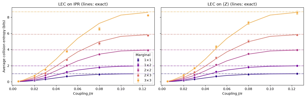
Beide Methoden beseitigen den größten Teil des Schadens: Die rohen Schätzwerte im vorherigen Diagramm sind viel zu zufällig, und die fehlergeminderten folgen den exakten Kurven. Die Unterschiede zeigen sich bei den größeren Marginalverteilungen.
Bei den kleinen Marginalverteilungen funktionieren beide Methoden. Bei der -Marginalverteilung liegt LEC auf deutlich näher.
Warum LEC auf dem IPR zu wenig Entropie liefert. Zu wenig Entropie bedeutet, dass der IPR zu groß ist: LEC auf dem IPR bläht ihn zu stark auf. Es nimmt an, dass Rauschen den Beitrag jedes zum IPR um denselben Faktor dämpft. Bei liegt jedes nahe , daher tragen alle Strings gleich viel bei, und die meisten Strings haben mittleres Gewicht: Von den 511 Strings einer -Marginalverteilung haben 252 das Gewicht 4 oder 5, und nur neun haben das Gewicht 1. Rauschen dämpft einen String umso stärker, je höher sein Gewicht ist (allein der Auslesefehler dämpft einen String vom Gewicht um ), daher wird der einzelne Faktor hauptsächlich durch die Dämpfung von Strings mittleren Gewichts bestimmt. Mit wachsendem zerfallen die mit höherem Gewicht am schnellsten, und der IPR wird immer mehr von Strings mit niedrigem Gewicht getragen, die das Rauschen weniger dämpft. Sie mit einem Faktor zu verstärken, der hauptsächlich an stärker gedämpften Strings gelernt wurde, bläht den IPR zu stark auf. Der Effekt wächst mit der Größe der Marginalverteilung, da eine größere Marginalverteilung einen breiteren Bereich an Gewichten hat. Er ist bei mittlerem am größten, nachdem sich die Mischung der Strings verschoben hat, der Überschuss des IPR über seinen Gleichverteilungswert aber noch ins Gewicht fällt.
Warum LEC auf in die andere Richtung irrt. Es skaliert jeden String mit seinem eigenen Faktor, daher beeinflusst die Verschiebung zwischen den Gewichten es nicht. Es nimmt nur an, dass jeder String seine Dämpfung bei beibehält. Mit wachsendem breitet sich jedes auf Operatoren mit höherem Gewicht aus, die mehr Rauschen aufnehmen als bei , sodass die Faktoren leicht unterkorrigieren und die Entropie etwas zu hoch ausfällt.
Die Vorhersage, die auf der Hardware zu testen ist, lautet also: Je größer die Marginalverteilung, desto deutlicher sollte LEC auf gewinnen. Auf der Hardware ist das Rauschen stärker und hat keine bekannte Form.
4. Im großen Maßstab ausführen
Das Hardware-Experiment läuft auf einem -Gitter mit vier Zyklen: 64 Qubits und 1.344 CZ-Gates in 48 Layern, bei neun Kopplungen. Gegenüber der Simulation ändern sich fünf Dinge:
-
Das Rauschen muss gelernt werden, was nur funktioniert, wenn die CZ-Layer fest sind.
-
Twirling verwandelt das Rauschen jedes Layers in einen Pauli-Kanal, der gelernt und verstärkt werden kann.
-
Dynamische Entkopplung (DD) schützt untätige Qubits.
-
Rauschverstärkung für PEA läuft im selben Job wie die Hauptdaten.
-
MPS-Simulationen bei kleinem liefern die klassischen Referenzen für die LEC-basierte Fehlerminderung.
Die Zellen, die ein Backend benötigen, laufen nur, wenn RUN_ON_HARDWARE auf True steht. MPS-Simulationen lassen sich erneut ausführen, wenn COMPUTE_MPS_REFERENCES auf True gesetzt ist. Die übrigen Zellen laufen hier.
# hardware run parameters:
num_cols_hw = num_rows_hw = 8
num_qubits_hw = num_cols_hw * num_rows_hw
num_cycles_hw = 4
couplings_hw = (
    np.array([0.005, 0.01, 0.02, 0.03, 0.05, 0.07, 0.09, 0.11, 0.125]) * np.pi
)
calibration_hw = 0  # J0 = 0.005π
disorder_hw = sample_disorder(
    num_cols_hw, num_rows_hw, np.random.default_rng(7)
)

# if running PEA:
noise_factors = np.array([1.0, 1.5, 2.0])  # PEA noise-amplification factors
Feste CZ-Layer
def compile_by_sublayer(
    num_cols,
    num_rows,
    coupling,
    num_cycles,
    disorder,
    pass_manager,
    layout=None,
    num_physical_qubits=None,
):
    # Compile each sublayer once and repeat it with barriers, so the CZ layers are the
    # same in every cycle and at every coupling. The registers are named explicitly
    # because register names enter Samplomatic's box hashes. Bits land in lattice order.
    num_qubits = num_cols * num_rows
    if layout is None:
        layout, num_physical_qubits = list(range(num_qubits)), num_qubits
    blocks = []
    for sublayer in disorder:
        block = QuantumCircuit(num_qubits)
        for (i, j), (h_i, h_j) in sublayer:
            heisenberg_gate(block, coupling, i, j, h_i, h_j)
        blocks.append(pass_manager.run(block))
    circuit = QuantumCircuit(
        QuantumRegister(num_physical_qubits, "q"),
        ClassicalRegister(num_qubits, "meas"),
    )
    neel_state(circuit, num_cols, num_rows, layout)
    for _ in range(num_cycles):
        for block in blocks:
            circuit.compose(block, inplace=True)
            circuit.barrier(layout)
    circuit.measure(layout, range(num_qubits))
    return circuit
Boxen für das Rauschlernen
Der Samplomatic-Boxing-Pass-Manager gruppiert dann jeden Circuit in Boxen: eine pro CZ-Layer und eine für die Messungen. Jede Box enthält einen Verweis auf das Rauschmodell, das sie braucht, sodass du prüfen kannst, dass alle Kopplungen dieselben Boxen teilen. Die nächste Zelle macht das für die -Circuits des Hardware-Laufs, ohne Backend zu CZ-Gates kompiliert, und gibt die Boxen aus, die das Rauschlernen charakterisieren wird.
from samplomatic import build
from samplomatic.transpiler import generate_boxing_pass_manager
from samplomatic.utils import find_unique_box_instructions

boxing_pass_manager = generate_boxing_pass_manager(
    enable_gates=True,  # twirl the CZ layers
    enable_measures=True,  # twirl the measurements
    inject_noise_targets="gates",  # PEA amplifies the noise of the CZ layers only
    inject_noise_strategy="uniform_modification",
)

def noise_refs(boxed_circuit):
    return sorted(
        annotation.ref
        for box in find_unique_box_instructions(boxed_circuit.data)
        for annotation in box.operation.annotations
        if hasattr(annotation, "ref")
    )

# The 8x8 hardware circuits, compiled to CZ gates on the lattice qubits (no backend needed)
compiled_8x8 = [
    compile_by_sublayer(
        num_cols_hw, num_rows_hw, c, num_cycles_hw, disorder_hw, pass_manager
    )
    for c in couplings_hw
]
boxed_8x8 = [boxing_pass_manager.run(circuit) for circuit in compiled_8x8]
assert all(
    noise_refs(b) == noise_refs(boxed_8x8[0]) for b in boxed_8x8
), "layers differ between couplings"
num_cz, depth = two_qubit_stats(compiled_8x8[0])
print(
    f"{num_qubits_hw} qubits: {num_cz} CZ gates in {depth} layers, for every coupling"
)
for box in find_unique_box_instructions(boxed_8x8[0].data):
    ops = box.operation.blocks[0].count_ops()
    print(
        f"{box.operation.num_qubits}-qubit box: {ops.get('cz', 0)} CZ, {ops.get('measure', 0)} measurements"
    )
print(
    f"All {len(boxed_8x8)} couplings share these {len(find_unique_box_instructions(boxed_8x8[0].data))} boxes"
)
64 qubits: 1344 CZ gates in 48 layers, for every coupling
64-qubit box: 32 CZ, 0 measurements
64-qubit box: 24 CZ, 0 measurements
64-qubit box: 32 CZ, 0 measurements
64-qubit box: 24 CZ, 0 measurements
64-qubit box: 0 CZ, 64 measurements
All 9 couplings share these 5 boxes
Die Circuits twirlen
In jeder Randomisierung setzt Samplomatic zufällige Pauli-Gates vor jede Box und die kompensierenden Gates danach, verschmolzen mit den benachbarten Ein-Qubit-Gates. Gemittelt über die Randomisierungen wird das Rauschen jedes Layers zu einem Pauli-Kanal, den NoiseLearnerV3 als dünnbesetztes Pauli-Lindblad-Modell lernen und den der PEA-Schritt verstärken kann. Das Mess-Twirling kippt vor dem Auslesen zufällig Bits. Die Kippungen werden in Software rückgängig gemacht, wodurch das Ausleserauschen symmetrisch wird; das ist die Grundlage der Ausleskorrektur (TREX).
Der Hardware-Workflow
Wähle die Qubits, kompiliere die Circuits, lerne dann das Rauschen und führe den Sweep aus. Diese Zellen sind hier ausgeschaltet.
Die Qubits wählen. Das quadratische Gitter von Nighthawk fasst das -Gitter ohne SWAP-Gates. Die Zelle bewertet jedes -Rechteck des Gitters anhand seiner gemeldeten CZ- und Auslesefehler und nimmt das beste.
def square_layouts(backend, side):
    # Every side x side rectangle of the square qubit grid that supports all bonds
    target = backend.target

    def has_cz(a, b):
        return (a, b) in target["cz"] or (b, a) in target["cz"]

    stride = next(
        s
        for s in (10, 12)
        if all(has_cz(q, q + s) for q in range(backend.num_qubits - s))
    )
    layouts = []
    for y0 in range(backend.num_qubits // stride - side + 1):
        for x0 in range(stride - side + 1):
            layout = [
                stride * (y0 + y) + x0 + x
                for y in range(side)
                for x in range(side)
            ]
            bonds = [
                bond
                for layer in brickwork_layers(side, side)
                for bond in layer
            ]
            if all(has_cz(layout[i], layout[j]) for i, j in bonds):
                layouts.append(((x0, y0), layout))
    return layouts

def layout_score(backend, layout, side, uses_per_bond):
    # Minus the summed log-fidelity of the bonds (each used uses_per_bond times) and readouts
    properties, target = backend.properties(), backend.target
    cz_errors = []
    for i, j in (
        bond for layer in brickwork_layers(side, side) for bond in layer
    ):
        pair = (
            (layout[i], layout[j])
            if (layout[i], layout[j]) in target["cz"]
            else (layout[j], layout[i])
        )
        cz_errors.append(properties.gate_error("cz", pair))
    readout_errors = [properties.readout_error(q) for q in layout]
    if max(cz_errors) >= 0.5 or max(readout_errors) >= 0.25:
        return np.inf  # an unusable qubit or bond
    return float(
        -uses_per_bond * np.log1p(-np.array(cz_errors)).sum()
        - np.log1p(-np.array(readout_errors)).sum()
    )

if RUN_ON_HARDWARE:
    from qiskit_ibm_runtime import QiskitRuntimeService

    def holds_lattice(backend):
        try:
            return bool(square_layouts(backend, num_cols_hw))
        except (KeyError, StopIteration):
            return False

    service = QiskitRuntimeService()
    candidates = [
        b
        for b in service.backends(operational=True, simulator=False)
        if holds_lattice(b)
    ]
    backend = min(candidates, key=lambda b: b.status().pending_jobs)
    score, origin, initial_layout = min(
        (
            layout_score(backend, layout, num_cols_hw, 3 * num_cycles_hw),
            origin,
            layout,
        )
        for origin, layout in square_layouts(backend, num_cols_hw)
    )
    print(f"{backend.name}: origin {origin}, score {score:.2f}")
Kompilieren. Dieselben Schritte wie oben auf den gewählten Qubits, gefolgt von build, das jeden geboxten Circuit in einen Template-Circuit und ein Samplex umwandelt, das Rezept zum Ziehen der Twirling-Gates und des eingespeisten Rauschens. DD wird zu den Templates hinzugefügt.
if RUN_ON_HARDWARE:
    from qiskit_ibm_runtime.executor.dynamical_decoupling import (
        generate_dd_pass_manager,
    )
    from qiskit_ibm_runtime.options import DynamicalDecouplingOptions

    # PEA structure functions:
    target_pass_manager = generate_preset_pass_manager(
        target=backend.target,
        optimization_level=3,
        initial_layout=initial_layout,
        routing_method="none",
        seed_transpiler=7,
    )
    boxed_hw = [
        boxing_pass_manager.run(
            compile_by_sublayer(
                num_cols_hw,
                num_rows_hw,
                coupling,
                num_cycles_hw,
                disorder_hw,
                target_pass_manager,
                layout=initial_layout,
                num_physical_qubits=backend.num_qubits,
            )
        )
        for coupling in couplings_hw
    ]
    assert all(noise_refs(b) == noise_refs(boxed_hw[0]) for b in boxed_hw)
    unique_boxes_hw = find_unique_box_instructions(boxed_hw[0].data)

    # DD pass:
    dd_pass_manager = generate_dd_pass_manager(
        backend,
        DynamicalDecouplingOptions(
            enable=True,
            sequence_type="XY4",
            scheduling_method="alap",
            extra_slack_distribution="middle",
            skip_reset_qubits=False,
        ),
    )
    templates = []
    for circuit in boxed_hw:
        template, samplex = build(circuit)
        templates.append((dd_pass_manager.run(template), samplex))
Das Rauschen lernen und den Sweep ausführen. Ein NoiseLearnerV3-Job lernt alle fünf Boxen: ein Pauli-Lindblad-Modell für jeden der vier CZ-Layer und das Ausleserauschen der Messbox. Dann enthält ein QuantumProgram alle neun Kopplungen. Jedes Element erhält sein Template, sein Samplex, die gelernten Rauschmodelle und drei Rauschskalen. Die Skala 0 sind die unverstärkten Daten für beide LEC-Methoden. Die Skalen 0,5 und 1 fügen für PEA 50 % und 100 % des gelernten Rauschens hinzu, wobei auf null Rauschen zurückextrapoliert wird. Das verbraucht etwa 40 Sekunden QPU-Zeit.
if RUN_ON_HARDWARE:
    from qiskit_ibm_runtime import Executor, NoiseLearnerV3, QuantumProgram

    # Learn the noise of the five boxes
    learner = NoiseLearnerV3(backend)
    learner.options.num_randomizations = 32
    learner.options.shots_per_randomization = 128
    # Up to 24 layer pairs, the depth of the 48-layer circuits
    learner.options.layer_pair_depths = [0, 1, 2, 4, 16, 24]
    learner_job = learner.run(unique_boxes_hw)
    print("Noise learning job:", learner_job.job_id())

    # Run the sweep, with the learned noise amplified by each of the noise factors
    noise_maps = learner_job.result().to_dict(
        instructions=unique_boxes_hw, require_refs=False
    )
    program = QuantumProgram(shots=200)
    for template, samplex in templates:
        program.append_samplex_item(
            template,
            samplex=samplex,
            samplex_arguments={
                "pauli_lindblad_maps": noise_maps,
                **{
                    f"noise_scales.{ref}": (noise_factors - 1).reshape(-1, 1)
                    for ref in noise_maps
                },
            },
            shape=(len(noise_factors), 200),  # noise scales x randomizations
        )
    executor_job = Executor(backend).run(program)
    print("Executor job:", executor_job.job_id())
    # Section 5 converts the results of these two jobs and saves them
5. Die Hardware-Daten
Dieser Abschnitt untersucht, wie die vorherigen Methoden bei echten Hardware-Daten eines Nighthawk-Prozessors abschneiden.
Den Lauf laden
Wenn RUN_ON_HARDWARE auf True steht, wandelt die nächste Zelle die Ergebnisse der beiden Jobs aus Abschnitt 4 um und speichert sie in data/hardware_run_new.npz, im selben Format wie der gespeicherte Lauf, sodass der neue Lauf später erneut analysiert werden kann. Andernfalls lädt sie den gespeicherten Lauf aus data/hardware_run.npz. Die Bits sind entlang der Qubit-Achse gepackt, um Platz zu sparen.
Falls der Kernel neu startet, während die Jobs laufen, reiche sie nicht erneut ein. Führe die Zellen vor dem letzten Aufruf in Abschnitt 4 erneut aus, prüfe, dass dieselben Qubits gewählt werden, und setze learner_job und executor_job auf service.job(job_id) mit den Job-IDs, die in Abschnitt 4 ausgegeben wurden.
if RUN_ON_HARDWARE:

    def unflip(item_result):
        # Undo the measurement twirling of an Executor item: flip back the bits that were flipped
        return item_result["meas"] ^ item_result["measurement_flips.meas"]

    learner_result = learner_job.result()
    raw_bits = [unflip(item) for item in executor_job.result()]

    # The learned readout map indexes the measured qubits in ascending physical order;
    # relabel it to lattice order
    measurement_box_index = next(
        k
        for k, box in enumerate(unique_boxes_hw)
        if "measure" in box.operation.blocks[0].count_ops()
    )
    measurement_box = next(
        inst
        for inst in boxed_hw[0].data
        if inst.operation.name == "box"
        and "measure" in inst.operation.blocks[0].count_ops()
    )
    measured = sorted(
        boxed_hw[0].find_bit(q).index for q in measurement_box.qubits
    )
    lattice_index = {physical: q for q, physical in enumerate(initial_layout)}
    readout_map = (
        learner_result[measurement_box_index]
        .to_pauli_lindblad_map()
        .apply_layout([lattice_index[p] for p in measured], num_qubits_hw)
    )

    # Save the run in the same format as the saved run, so it can be analyzed again later
    terms = readout_map.to_sparse_list()
    np.savez_compressed(
        "data/hardware_run_new.npz",
        bits=np.packbits(np.stack(raw_bits), axis=-1, bitorder="little"),
        labels=np.array([label for label, _, _ in terms]),
        indices=np.concatenate(
            [np.asarray(support) for _, support, _ in terms]
        ),
        rates=np.array([rate for _, _, rate in terms]),
        physical_qubits=np.array(initial_layout),
        couplings_over_pi=couplings_hw / np.pi,
        noise_factors=noise_factors,
    )
else:
    saved = np.load(
        "data/hardware_run.npz"
    )  # or data/hardware_run_new.npz, for a new run
    raw_bits = list(
        np.unpackbits(
            saved["bits"], axis=-1, count=num_qubits_hw, bitorder="little"
        ).astype(bool)
    )
    labels = [str(label) for label in saved["labels"]]
    indices = np.split(
        saved["indices"], np.cumsum([len(label) for label in labels])[:-1]
    )
    readout_map = PauliLindbladMap.from_sparse_list(
        list(zip(labels, indices, saved["rates"])), num_qubits_hw
    )

print(f"{len(raw_bits)} couplings, bits per coupling: {raw_bits[0].shape}")
print(
    f"Readout noise: {readout_map.num_terms} terms on {readout_map.num_qubits} qubits"
)
9 couplings, bits per coupling: (3, 200, 200, 64)
Readout noise: 64 terms on 64 qubits
Klassische Referenzen
Beide LEC-Methoden benötigen die idealen Marginalverteilungen bei , und zum Testen braucht man ideale Werte bei den zurückgehaltenen Kopplungen und . Diese stammen aus Matrix-Produkt-Zustands-Simulationen (MPS), gespeichert für jede Platzierung jeder Marginalform auf dem Gitter, wie im Paper, und für jeden nicht überlappenden -Block bei . Bei konvergieren sie bei Bonddimension . Bei und verwenden sie , und bei ändern sie sich für -Marginalverteilungen gegenüber noch um bis zu etwa 13 %, behandle sie dort also als Näherung. Die nächste Zelle berechnet sie, wenn COMPUTE_MPS_REFERENCES auf True steht, was etwa 18 Minuten dauert, und lädt andernfalls die gespeicherten Ergebnisse, indiziert nach Kopplungsindex, Bonddimension und Marginalverteilung.
# Every placement of every shape on the 8x8 lattice
positions = {
    label: all_positions(shape, num_cols_hw, num_rows_hw)
    for label, shape in patch_shapes.items()
}
reference_settings = [
    (calibration_hw, 32),
    (calibration_hw, 64),
    (1, 128),
    (2, 64),
    (2, 128),
]  # (coupling, χ)

if COMPUTE_MPS_REFERENCES:

    def mps_patch_probabilities(coupling, patches, bond_dimension):
        # Distributions of the given marginals after the 8x8 circuit, from an MPS simulation
        simulator = AerSimulator(
            method="matrix_product_state",
            matrix_product_state_max_bond_dimension=bond_dimension,
            matrix_product_state_truncation_threshold=1e-12,
        )
        circuit = heisenberg_floquet_circuit(
            num_cols_hw,
            num_rows_hw,
            coupling,
            num_cycles_hw,
            disorder_hw,
            measure=False,
        )
        circuit = generate_preset_pass_manager(
            optimization_level=1, basis_gates=["cx", "u"], seed_transpiler=7
        ).run(circuit)
        for label, qubits in patches.items():
            circuit.save_probabilities(qubits, label=label)
        data = simulator.run(circuit, shots=1).result().data(0)
        return {label: np.asarray(data[label]) for label in patches}

    placements = {
        f"{label} {k}": qubits
        for label, patch_list in positions.items()
        for k, qubits in enumerate(patch_list)
    }
    tiles = {
        f"site {q}": [q] for q in range(num_qubits_hw)
    } | {  # for the lattice map at J0
        f"block {x},{y}": patch_qubits((2 * x, 2 * y), (2, 2), num_cols_hw)
        for y in range(num_rows_hw // 2)
        for x in range(num_cols_hw // 2)
    }
    computed = {}
    for index, chi in reference_settings:
        targets = (
            placements | tiles
            if (index, chi) == (calibration_hw, 64)
            else placements
        )
        for key, p in mps_patch_probabilities(
            couplings_hw[index], targets, chi
        ).items():
            computed[f"{index}/{chi}/{key}"] = p
    np.savez_compressed("data/mps_references_all.npz", **computed)
    saved = computed
else:
    saved = np.load("data/mps_references_all.npz")

references = {}  # (coupling index, bond dimension) -> {marginal key: distribution}
for name in saved:
    index, chi, key = name.split("/", 2)
    references.setdefault((int(index), int(chi)), {})[key] = saved[name]
Datenqualität: fehlerhafte Koppler / Qubits
Sieh dir zuerst die niedrigste Kopplung an, bei der die Erwartungswerte nahe am Néel-Schachbrettmuster liegen sollten.
# <Z> of every site at J0: the MPS reference, and the hardware data at noise factor 1
z_reference = np.array(
    [
        parities_from_probabilities(
            references[(calibration_hw, 64)][f"site {q}"]
        )[0]
        for q in range(num_qubits_hw)
    ]
)
z_measured = 1 - 2 * raw_bits[calibration_hw][0].mean(axis=(0, 1))
fig, axes = plt.subplots(1, 2, figsize=(11, 4.6), layout="constrained")
fig.get_layout_engine().set(wspace=0.12)  # white space between the two panels
edges = np.arange(num_cols_hw + 1) - 0.5
for ax, values, title in zip(
    axes, (z_reference, z_measured), ("MPS reference", "Hardware")
):
    mesh = ax.pcolormesh(
        edges,
        edges,
        values.reshape(num_rows_hw, num_cols_hw),
        cmap="RdBu_r",
        vmin=-1,
        vmax=1,
        edgecolors="white",
    )
    ax.set_aspect("equal")
    ax.invert_yaxis()
    ax.set_xticks([])
    ax.set_yticks([])
    ax.set_title(
        f"{title}, $J_0 = {couplings_hw[calibration_hw] / np.pi:g}\\pi$"
    )
fig.colorbar(
    mesh, ax=axes, shrink=0.8, label=r"$\langle Z \rangle$ of each site"
)
plt.show()

Frage. Was fällt dir auf der Hardware-Karte auf?
Antwort
Die blassen Stellen, die fast ihr gesamtes Signal verloren haben, obwohl der Zustand bei nahe am Néel-Zustand liegt. Sie sind wichtig, weil LEC durch das Signal teilt, das bei übrig bleibt: Ein Qubit mit fast keinem Signal liefert einen riesigen, verrauschten Korrekturfaktor, und einige wenige solcher Qubits können jede Marginalverteilung dominieren, die sie enthält.
Eine Regel, die nur die Daten verwendet: Ein Qubit ist fehlerhaft, wenn sein Ein-Qubit-IPR bei innerhalb von von liegt, dem Wert für ein vollständig gemischtes Qubit. Da der IPR eines Qubits ist, markiert das Qubits mit . Marginalverteilungen, die eine markierte Stelle enthalten, werden unten ausgelassen.
site_iprs = np.array(
    [
        ipr_from_shots(raw_bits[calibration_hw][0][:, :, [q]])
        for q in range(num_qubits_hw)
    ]
)
# |IPR - 1/2| < 0.25**2 / 2 is the same as |<Z>| < 0.25
flagged = {
    q for q in range(num_qubits_hw) if abs(site_iprs[q] - 0.5) < 0.25**2 / 2
}
print(
    f"Median single-qubit IPR at J0: {np.median(site_iprs):.2f}; flagged lattice sites {sorted(flagged)}"
)
Median single-qubit IPR at J0: 0.77; flagged lattice sites [19, 24, 25, 27, 32]
Die zu mittelnden Marginalverteilungen auswählen
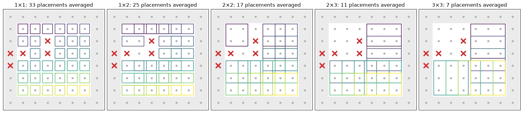
Die nächste Zelle zeigt, welche Platzierungen jeder Form in die folgenden Mittelwerte eingehen: jede Platzierung im Inneren des Gitters ohne markierte Stelle (rote Kreuze). Platzierungen, die den Rand berühren (schattiert), werden ausgelassen. Randqubits haben weniger Bindungen und verwirbeln daher langsamer. Für sich gemittelt, überschreiten sie den Übergang für jede Form und Methode einen vollen Schritt in später als Platzierungen im Inneren. Jede gemittelte Platzierung hat ihre eigene Box, nach Platzierung eingefärbt.
def touches_edge(qubits):
    # Whether a placement includes a site on the edge of the lattice
    return any(
        q % num_cols_hw in (0, num_cols_hw - 1)
        or q // num_cols_hw in (0, num_rows_hw - 1)
        for q in qubits
    )

# The placements of each shape that enter the averages: in the bulk, and without a flagged site
kept_placements = {
    label: [
        k
        for k, qubits in enumerate(patch_list)
        if not touches_edge(qubits) and not set(qubits) & flagged
    ]
    for label, patch_list in positions.items()
}
placement_cmap = plt.get_cmap("viridis")
fig, axes = plt.subplots(
    1, len(positions), figsize=(17, 4.4), layout="constrained"
)
for ax, (label, patch_list) in zip(axes, positions.items()):
    width, height = patch_shapes[label]
    for q in range(num_qubits_hw):
        x, y = q % num_cols_hw, q // num_cols_hw
        if touches_edge([q]):  # shade the edge of the lattice
            ax.add_patch(
                plt.Rectangle(
                    (x - 0.5, y - 0.5), 1, 1, color="0.92", zorder=0
                )
            )
        ax.plot(x, y, "o", color="0.7", ms=4, zorder=1)
    kept = kept_placements[label]
    for i, k in enumerate(kept):
        qubits = patch_list[k]
        x0, y0 = (
            qubits[0] % num_cols_hw,
            qubits[0] // num_cols_hw,
        )  # top-left site of the placement
        ax.add_patch(
            plt.Rectangle(
                (x0 - 0.4, y0 - 0.4),
                width - 0.2,
                height - 0.2,
                fill=False,
                lw=1.2,
                ec=placement_cmap(i / max(len(kept) - 1, 1)),
                zorder=2,
            )
        )
    for q in flagged:
        ax.plot(
            q % num_cols_hw,
            q // num_cols_hw,
            "x",
            color="#d62728",
            ms=11,
            mew=3,
            zorder=3,
        )
    ax.set_xlim(-0.6, num_cols_hw - 0.4)
    ax.set_ylim(num_rows_hw - 0.4, -0.6)
    ax.set_aspect("equal")
    ax.set_xticks([])
    ax.set_yticks([])
    ax.set_title(f"{label}: {len(kept)} placements averaged")
plt.show()
PEA
Die dritte Methode braucht keine klassische Referenz. Nimm für jede Parität die Werte bei den Rauschfaktoren 1, 1,5 und 2, teile die gelernte Auslesedämpfung heraus (TREX), passe eine Exponentialfunktion im Rauschfaktor an und extrapoliere auf null Rauschen. Paritäten, die das Vorzeichen wechseln oder nahezu null sind, erhalten eine Geradenanpassung. Das Subtrahieren der Varianz braucht eine verlässliche Schätzung derselben, was für rohe und skalierte Paritäten einfach ist, nicht aber für die Ausgabe einer nichtlinearen Anpassung mit Clipping und Rückfalllösungen. PEA verwendet deshalb den anderen Standardweg, um den Bias eines Quadrats zu entfernen. Extrapoliere jede Hälfte der Randomisierungen getrennt und multipliziere die beiden unabhängigen Schätzungen.
def readout_fidelity(support):
    # Damping of <Z_S> by the learned readout noise
    pauli = QubitSparsePauli.from_sparse_label(
        ("Z" * len(support), list(support)), num_qubits_hw
    )
    return readout_map.pauli_fidelity(pauli)

def extrapolate_to_zero(values):
    # Fit a * exp(b * factor) to each column of values (noise factors first), or a line
    # where the values change sign or come within 1e-3 of zero
    result = np.polynomial.polynomial.polyfit(noise_factors, values, 1)[0]
    sign = np.sign(values[0])
    usable = np.all(np.sign(values) == sign, axis=0) & (
        np.abs(values).min(axis=0) > 1e-3
    )
    if usable.any():
        log_fit = np.polynomial.polynomial.polyfit(
            noise_factors, np.log(np.abs(values[:, usable])), 1
        )
        result[usable] = sign[usable] * np.exp(log_fit[0])
    return result

def pea_ipr(parities, fidelities, num_patch):
    # parities has shape (noise factors, randomizations, supports). Extrapolate the two
    # halves of the randomizations separately; their errors are independent, so the
    # product of the two estimates of each parity has no shot-noise bias
    def zero_noise(p):
        # A parity cannot exceed 1 in magnitude, so cap the extrapolated values there
        return np.clip(
            extrapolate_to_zero(p.mean(axis=1) / fidelities), -1, 1
        )

    half = parities.shape[1] // 2
    first, second = (
        zero_noise(parities[:, :half]),
        zero_noise(parities[:, half:]),
    )
    return float((1 + np.dot(first, second)) / 2**num_patch)
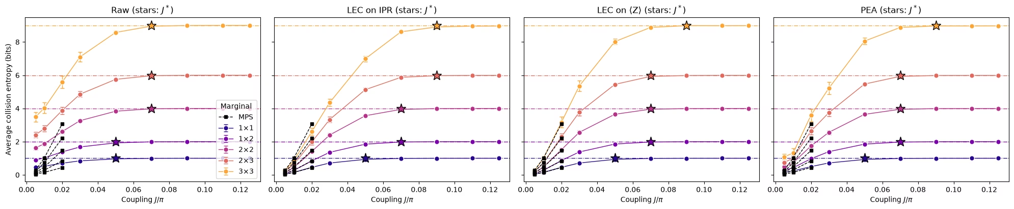
Alle vier Schätzungen und die Übergänge
Die nächste Funktion berechnet die rohen Schätzungen sowie die Schätzungen mit LEC auf dem IPR, LEC auf und PEA für den IPR einer Marginalposition bei jeder Kopplung. Sie schätzt außerdem das Shot-Rauschen jeder Schätzung durch Bootstrapping der Randomisierungen. Die Zelle führt sie für jede Platzierung aus, die in die Mittelwerte eingeht, was etwa anderthalb Minuten dauert.
def estimate_iprs(qubits, key):
    # Raw, LEC-on-IPR, LEC-on-<Z>, and PEA IPRs of one marginal position at every coupling,
    # with the shot noise of each from a bootstrap over the randomizations
    n = len(qubits)
    supports = parity_supports(qubits)
    # Parities with shape (noise factors, randomizations, supports), per coupling
    parities = [
        np.stack([parity_expectation_values(b, supports) for b in bits])
        for bits in raw_bits
    ]
    patch_bits = [
        bits[0][:, :, qubits] for bits in raw_bits
    ]  # noise factor 1
    values, errors = lec_estimates(
        patch_bits,
        [p[0] for p in parities],
        references[(calibration_hw, 64)][key],
        calibration_hw,
        n,
    )
    fidelities = np.array([readout_fidelity(s) for s in supports])

    def pea_statistic(p):
        return pea_ipr(p, fidelities, n)

    values["raw"] = [ipr_from_shots(b) for b in patch_bits]
    errors["raw"] = [bootstrap_error(ipr_from_shots, b) for b in patch_bits]
    values["PEA"] = [pea_statistic(p) for p in parities]
    errors["PEA"] = [
        bootstrap_error(pea_statistic, p, axis=1) for p in parities
    ]  # randomizations are axis 1
    return {m: np.array(v) for m, v in values.items()}, {
        m: np.array(e) for m, e in errors.items()
    }

methods = ["LEC on IPR", "LEC on ⟨Z⟩", "PEA"]
method_colors = {
    "LEC on IPR": "#2a78d6",
    "LEC on ⟨Z⟩": "#1baf7a",
    "PEA": "#eb6834",
}
iprs, ipr_errors = {}, {}
for label, patch_list in positions.items():
    for k in kept_placements[label]:
        iprs[label, k], ipr_errors[label, k] = estimate_iprs(
            patch_list[k], f"{label} {k}"
        )
print(f"{len(iprs)} clean marginal positions")
93 clean marginal positions
def crossover_coupling(couplings, entropies, haar, tolerance=0.1):
    # Smallest coupling whose entropy is within tolerance of the random-state value
    for coupling, entropy in zip(couplings, entropies):
        if entropy >= haar - tolerance:
            return coupling
    return None

def reference_ipr(index, chi, key):
    # IPR of the MPS distribution of a marginal
    return float((references[(index, chi)][key] ** 2).sum())

mps_settings = [
    (calibration_hw, 64),
    (1, 128),
    (2, 128),
]  # (coupling index, bond dimension)
panels = ["raw", *methods]

# Average IPR of every shape over its clean placements, then the entropy and the crossover
hw_entropies = {
    method: {} for method in panels
}  # per method and shape: average entropy and its error
crossovers = {method: {} for method in panels}
mps_entropies = {}  # per shape: MPS entropy, averaged over the same placements, at mps_settings
for label, patch_list in positions.items():
    haar = haar_entropy(len(patch_list[0]), num_qubits_hw)
    keys = [(shape, k) for (shape, k) in iprs if shape == label]
    mps_entropies[label] = [
        collision_entropy(
            np.mean([reference_ipr(j, chi, f"{label} {k}") for _, k in keys])
        )
        for j, chi in mps_settings
    ]
    for method in panels:
        ipr, ipr_error = average_ipr(
            [iprs[key][method] for key in keys],
            [ipr_errors[key][method] for key in keys],
        )
        entropy = collision_entropy(ipr)
        hw_entropies[method][label] = (entropy, ipr_error / (ipr * np.log(2)))
        crossovers[method][label] = crossover_coupling(
            couplings_hw, entropy, haar
        )
fig, axes = plt.subplots(
    1, len(panels), figsize=(5 * len(panels), 4.2), sharey=True
)
for (label, patch_list), color in zip(positions.items(), colors):
    haar = haar_entropy(len(patch_list[0]), num_qubits_hw)
    for ax, method in zip(axes, panels):
        entropy, error = hw_entropies[method][label]
        ax.errorbar(
            couplings_hw / np.pi,
            entropy,
            yerr=error,
            fmt="o-",
            color=color,
            mec="white",
            ms=7,
            lw=1,
            capsize=3,
            label=label,
        )
        ax.plot(
            couplings_hw[[j for j, _ in mps_settings]] / np.pi,
            mps_entropies[label],
            "s--",
            color="black",
            ms=4,
            lw=1,
            label="MPS" if label == "3×3" else None,
            zorder=4,
        )
        ax.axhline(haar, color=color, ls="dashdot", lw=0.9)
        if crossovers[method][label]:
            ax.plot(
                crossovers[method][label] / np.pi,
                haar,
                "*",
                ms=14,
                color=color,
                mec="black",
                zorder=3,
            )
for ax, method in zip(axes, panels):
    ax.set_title(f"{'Raw' if method == 'raw' else method} (stars: $J^*$)")
    ax.set_xlabel("Coupling $J/\\pi$")
axes[0].set_ylabel("Average collision entropy (bits)")
axes[0].legend(title="Marginal", loc="lower right")
fig.tight_layout()
plt.show()
Zusammenfassung
Was nötig war, um ein Experiment dieser Größe auszuführen:
-
Circuits, deren Struktur nicht von abhängt, Sublayer für Sublayer kompiliert, sodass ein Rauschmodell den gesamten Sweep abdeckt.
-
Schätzer, die mit Bitstrings arbeiten: Paarzählung für den IPR einer Marginalverteilung und die Parseval-Form, bei der von jeder quadrierten Parität die Varianz subtrahiert wird, wenn die Eingaben fehlergeminderte Erwartungswerte sind.
-
Ein günstiger klassischer Anker: Der ideale Zustand bei kleinem kalibriert das Rauschen, und zurückgehaltene Kopplungen testen die Kalibrierung. Jedes einzeln zu kalibrieren, statt den IPR als Ganzes, ist es, was die großen Marginalverteilungen in Einklang bringt.
-
IBM-Werkzeuge für die Schwerarbeit: Samplomatic-Boxen und Twirling,
NoiseLearnerV3, dynamische Entkopplung und einExecutor-Job mit Rauschverstärkung für PEA. -
Datenqualitätsprüfungen, die nur die Daten verwenden.
Nächste Schritte. Um bei der Fehlerminderung weiterzugehen, sieh dir die Tutorials Probabilistic error amplification und PEC with shaded lightcones an.